3.15.1. TI Deep Learning (TIDL)
3.15.1.1. Introduction
3.15.1.1.1. Deep Learning Inference in Embedded Device
TIDL brings deep learning to the edge by enabling applications to leverage TI’s proprietary, highly optimized CNN/DNN implementation on the EVE and C66x DSP compute engines. TIDL initially targets use cases with 2D (typically vision) data on AM57x SoCs. There are not fundamental limitations preventing the use of TIDL for 1D or 3D input data blobs.
TIDL is a set of open-source Linux software packages and tools enabling offload of Deep Learning (inference only) compute workloads from Arm cores to hardware accelerators such as EVE and/or C66x DSP. The objective for TIDL is to hide complexity of a heterogeneous device for Machine Learning/Neural network applications, and help developers focus on their specific requirements. In this way, Arm cores are freed from heavy compute load of Deep Learning task and can be used for other roles in your application. This also allows to use traditional Computer Vision (via OpenCV) augmenting Deep Learning algorithms.
At the moment, TIDL software primarily enables Convolution Neural Network inference, using offline pre-trained models, stored in device file-system (no training on target device). Models trained using Caffe or Tensorflow-slim frameworks can be imported and converted (with provided import tool) for efficient execution on TI devices.
Additional performance benefits can be achieved by doing training using Caffe-Jacinto fork of Caffe, which includes functions for making convolution weight tensor sparse, thus giving opportunity for 3x-4x performance boost of convolutions layers.
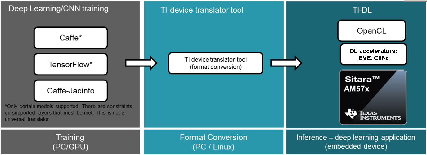
Fig. 3.6 Deep Learnining development flow on AM57xx devices
3.15.1.1.2. Application space
Current version of TIDL software is targeting Computer Vision Deep Learning applications. Example applications include vision computers, barcode readers, machine vision cameras, industrial automation systems, optical inspection systems, industrial robots, currency counters, occupancy detectors, smart appliances and unmanned vehicles. In these cases color image tensors (Width x Height x 3, for BGR planes) are typically used, but it is possible to use other data types (E.g. gray scale and depth plane: Width x Height x 2 tensor)
Based on model and task, TIDL input data are similar, but output data will vary based on task:
| Task | Output Data |
|---|---|
| Image Classification | 1D vector with likelihood of class presence. Top ranking indicates class winner (i.e. object of data class appears in input) |
| Image Pixel Segmentation | 2D matrix: Width x Height, with each cell set to integer value from 0 to max_class_index that model can discriminate |
| Image Object Detection | list of tuples. Each tuple includes class index, probability of detection, upper left corner (xmin,ymin), width and height of bounding box |
Additional examples covering other application areas (speech, audio, predictive maintenance), are in the road map. Apart from Convolution Network topologies, support for RNN/LSTM layers and topologies, targetting processing of sequential data, are planned in future releases.
3.15.1.1.3. Supported Devices
TIDL software is intended for AM57xx Sitara devices, that either have DSP or EVE, or both accelerators:
- AM5749 (2xEVEs + 2xC66x DSPs)
- AM5746 (2xC66x DSPs)
- AM572x (2xC66x DSPs)
- AM571x (1xC66x DSP)
- AM5706 (1xC66x DSP)
- AM5708 (1xC66x DSP)
3.15.1.1.4. TIDL API framework abstracts multicore operation
Current implementation of TIDL API provides following important features:
Running a network on individual EVE subsystem or C66x DSP core
- Multiple networks on different EVEs/DSPs can run concurrently
We can run concurrently as many different networks as we have available accelerators. Single unit of task execution is complete network, i.e. it is typically executed from start to end on only one EVE or DSP.
- Splitting the network layers between available accelerators (EVE subsystem and/or C66x cores)
For certain networks (JDetNet is one example), it is beneficial to use concept of layer groups. One layer group runs on EVE and another on DSP. There are few layers which runs faster on DSP: SoftMax, Flatten and Concat layers. So in this case we are using DSP+EVE for single network.
- Same TIDL API based application code can run on EVE or DSP accelerator
This can be achieved just by modifying a device type parameter More details in Introduction to Programming Model
Maximum number of inference tasks on AM5749 is 4 (2xEVE and 2xDSP), whereas on AM5728 maximum number of tasks is 2 (2xDSP). All TIDL related memory buffers (~64MB per core: network configuration parameters, layer activations, input/output buffers) must fit into CMEM section.
3.15.1.2. Verified networks topologies
It is necessary to understand that TIDL is not verified against arbitrary network topology. Instead, we were focused on verification of layers and network topologies that make sense to be executed on power-constraint embedded devices. Some networks are too complex for power budget of few watts. So focus is put on networks that are not extremely computationally intensive and also not having very high memory requirements.
TIDL supports topologies described in the following framework formats:
- Caffe
- TensorFlow
- TensorFlow Lite
- ONNX
The following topologies have been verified with TIDL software:
- Jacinto11 (similar to ResNet10), classification network
- JSeg21, pixel level segmentation network
- JDetNet, (similar to SSD-300/512), object detection network
- SqueezeNet
- InceptionV1
- InceptionV3
- MobileNetV1
- MobileNetV2
- Resnet18V1
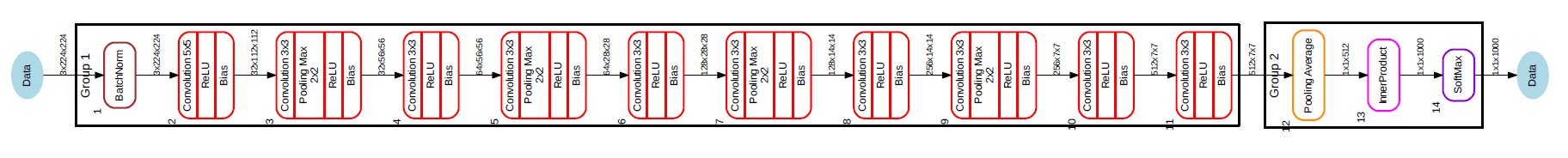
Here are the graphs (created using TIDL viewer tool) of first three:
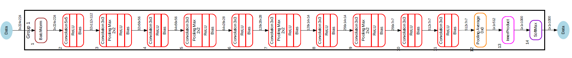
Fig. 3.7 Figure Jacinto11 (resnet10 motivated)

Fig. 3.8 Figure JSeg21 (SegNet motivated)
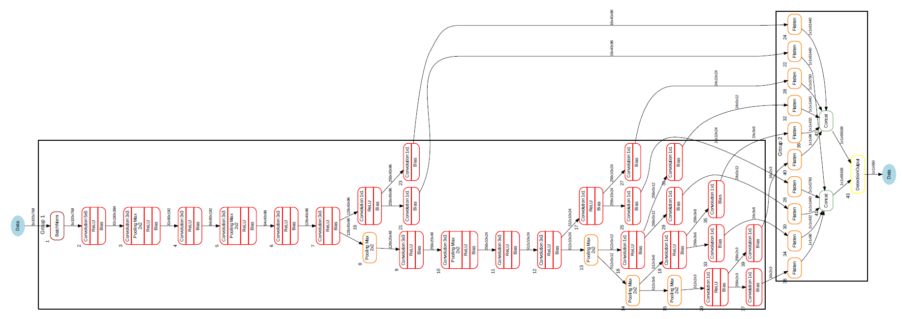
Fig. 3.9 Figure JDetNet (SSD-300/512 motivated)
Other network topologies are possible but they need to be verified. Majority of layers required (for inference only!) for classification, segmentation and detection tasks are implemented, though in some cases with certain parameter related constraints.
3.15.1.2.1. Neural network layers supported by TIDL
The following layer types/Inference features are supported:
- Convolution Layer
- Pooling Layer (Average and Max Pooling)
- ReLU Layer
- Element Wise Layer (Add, Max, Product)
- Inner Product Layer (Fully Connected Layer)
- Soft Max Layer
- Bias Layer
- Deconvolution Layer
- Concatenate layer
- ArgMax Layer
- Scale Layer
- PReLU Layer
- Batch Normalization layer
- ReLU6 Layer
- Crop layer
- Slice layer
- Flatten layer
- Split Layer
- Detection Output Layer
During import process (described later), some operators or layers in a network model will be coalesced or converted into TIDL layers listed above. The supported operators/layers for Tensorflow/TensorFlow Lite/ONNX/Caffe are listed below.
Supported TensorFlow operators and the corresponding TIDL layers:
| TensorFlow Operator | TIDL Layer |
|---|---|
| Placeholder | TIDL_DataLayer |
| Conv2D | TIDL_ConvolutionLayer |
| DepthwiseConv2dNative | TIDL_ConvolutionLayer |
| BiasAdd | TIDL_BiasLayer |
| Add | TIDL_EltWiseLayer |
| Mul | TIDL_ScaleLayer |
| FusedBatchNorm | TIDL_BatchNormLayer |
| Relu | TIDL_ReLULayer |
| Relu6 | TIDL_ReLULayer |
| MaxPool | TIDL_PoolingLayer |
| AvgPool | TIDL_PoolingLayer |
| ConcatV2 | TIDL_ConcatLayer |
| Slice | TIDL_SliceLayer |
| Squeeze | See note below |
| Reshape | See note below |
| Softmax | TIDL_SoftMaxLayer |
| Pad | TIDL_PadLayer |
| Mean | TIDL_PoolingLayer |
Supported TensorFlow Lite operators and the corresponding TIDL layers:
| TensorFlow Operator | TIDL Layer |
|---|---|
| Placeholder | TIDL_DataLayer |
| CONV_2D | TIDL_ConvolutionLayer |
| TRANSPOSE_CONV | TIDL_Deconv2DLayer |
| DEPTHWISE_CONV_2D | TIDL_ConvolutionLayer |
| ADD | TIDL_EltWiseLayer |
| MUL | TIDL_ScaleLayer |
| RELU | TIDL_ReLULayer |
| RELU6 | TIDL_ReLULayer |
| MAX_POOL_2D | TIDL_PoolingLayer |
| AVERAGE_POOL_2D | TIDL_PoolingLayer |
| CONCATENATION | TIDL_ConcatLayer |
| RESHAPE | See note below |
| SOFTMAX | TIDL_SoftMaxLayer |
| ARG_MAX | TIDL_ArgMaxLayer |
| PAD | TIDL_PadLayer |
| MEAN | TIDL_PoolingLayer |
| FULLY_CONNECTED | TIDL_InnerProductLayer |
Note
- “Reshape” and “Squeeze” are supported by being coalesced into other layers:
- If “Reshape” immediately follows “Squeeze”, they both are coalesced into TIDL_FlattenLayer.
- If “Reshape” immediately follows “AvgPool”, “Reshape” is coalesced into TIDL_PoolingLayer.
- If “Reshape” immediately follows TIDL_InnerProductLayer, it is coalesced into TIDL_InnerProductLayer.
- “Conv2D” is converted to TIDL_InnerProductLayer if:
- convolution kernel is 1x1 and input is one dimension vector,
- input is TIDL_PoolingLayer with average pooling, and
- output is TIDL_SoftMaxLayer or TIDL_FlattenLayer.
Supported ONNX operators and the corresponding TIDL layers:
| ONNX Operator | TIDL Layer |
|---|---|
| Conv | TIDL_ConvolutionLayer |
| MaxPool | TIDL_PoolingLayer |
| AveragePool | TIDL_PoolingLayer |
| GlobalAveragePool | TIDL_PoolingLayer |
| Relu | TIDL_ReLULayer |
| Concat | TIDL_ConcatLayer |
| Reshape | See note below |
| Transpose | See note below |
| Add | TIDL_EltWiseLayer |
| Sum | TIDL_EltWiseLayer |
| ArgMax | TIDL_ArgMaxLayer |
| BatchNormalization | TIDL_BatchNormLayer |
| Gemm | TIDL_InnerProductLayer |
| Softmax | TIDL_SoftMaxLayer |
| Dropout | TIDL_DropOutLayer |
Note
- If “Reshape” is followed by “Transpose” and then followed by “Reshape”, then they are coalesced into TIDL_FlattenLayer.
- If “Reshape” immediately follows “AvgPool”, “Reshape” is coalesced into TIDL_PoolingLayer.
- If “Reshape” immediately follows inner product layer, “Reshape” is coalesced into TIDL_InnerProductLayer.
Supported Caffe layer types and the corresponding TIDL layers:
| Caffe Layer Type | TIDL Layer |
|---|---|
| Concat | TIDL_ConcatLayer |
| Convolution | TIDL_ConvolutionLayer |
| Pooling | TIDL_PoolingLayer |
| ReLU/LRN | See note below |
| PReLU | TIDL_BatchNormLayer |
| Dropout | TIDL_DropOutLayer |
| Softmax | TIDL_SoftMaxLayer |
| Deconvolution | TIDL_Deconv2DLayer |
| Argmax | TIDL_ArgMaxLayer |
| Bias | TIDL_ConvolutionLayer |
| Eltwise | TIDL_EltWiseLayer |
| BatchNorm | TIDL_BatchNormLayer |
| Scale | TIDL_BatchNormLayer |
| InnerProduct | TIDL_InnerProductLayer |
| Split | TIDL_SplitLayer |
| Slice | TIDL_SliceLayer |
| Crop | TIDL_CropLayer |
| Flatten | TIDL_FlattenLayer |
| Permute | See note |
| PriorBox | See note |
| Reshape | See note |
| DetectionOutput | TIDL_DetectionOutputLayer |
Note
- “ReLU/LRN” can be merged into TIDL_ConvolutionLayer, TIDL_EltWiseLayer, TIDL_InnerProductLayer, or TIDL_BatchNormLayer.
- If “Permute” is followed by “Flatten”, “Permute” is merged into TIDL_FlattenLayer. This is only applicable for SSD network.
- If “PriorBox” is followed by “DetectionOutput” or “Concat”, “PriorBox” is merged into TIDL_DetectionOutputLayer or TIDL_ConcatLayer.
- If “Reshape” is followed by “Softmax”, “Reshape” is merged into TIDL_SoftMaxLayer. This is only applicable for SSD network.
3.15.1.2.2. Constraints on layer parameters
Layers in current release of TIDL Lib have certain parameter related constraints:
- Convolution Layer
- Kernel size up to 7x7
- Dilation vaild for parameter values of: 1,2,4
- Stride values of 1 and 2 are supported.
- Dense convolution flow is supported for only 1x1 and 3x3 kernels with stride = 1 and dilation =1
- Maximum number of input and output channel supported: 1024.
- Deconvolution Layer
- Number of groups shall be equal to the number of channels
- Only supported stride value is 2
- Arg Max
- Up to 15 input channels are supported for EVE core and up to 6 channels are supported for DSP core
- out_max_val = false and top_k = 1 (Defaults) and axis = 1 (Supported only across channel)
- InnerProductLayer
- Maximum input and output Nodes supported are 4096
- The input data has to be flattened (That is C =1 and H =1 for the input data)
- A flatten layer can be used before this layer in C > 1 and H > 1
- A global average pooling also can be used to flatten the output
- Input size has to be multiple of 8, because DSP implementation of the layer does aligned 8-byte double word loads
- Spatial Pooling Layer
- Average and Max Pooling are supported with stride 1, 2, 4 and kernel sizes of 2x2,3x3,4x4 etc. STOCHASTIC Pooling not supported
- Global Pooling supported for both Average and Max. The output data N=1 and H =1. The output W will be Updated with input ‘N’
- Global Pooling can operate on feature maps up to 64x64 size.
- BiasLayer
- Only one scalar bias per channel is supported.
- CancatLayet
- Concatenate is only supported across channel (axis = 1; default).
- CropLayer
- Only Spatial crop is supported (axis = 2; default).
- FlattenLayer
- Keeps ‘N’ unchanged. Makes C=1 and H=1
- ScaleLayer
- Only one scalar scale and bias per channel is supported.
- SliceLayer
- Slice is only supported across channel (axis = 1; default).
- SoftmaxLayer
- The input data has to be flattened (That is C =1 and H =1 for the input data)
- SSD
- Only Caffe-Jacinto based SSD network is validated.
- Reshape, Permute layers are supported only in the context of SSD network.
- “share_location” has to be true
- Tested with 4 and 5 heads.
- SaveOutputParameter is ignored in TIDL inference.
- Code_type is only tested with CENTER_SIZE.
- Tensorflow
- Only Slim based models are validated. Please refer InceptionNetV1 and mobilenet_1.0 from below as examples for building your models.
- TF-Slim: https://github.com/tensorflow/models/tree/master/research/slim
3.15.1.3. Examples and Demos
3.15.1.3.1. TIDL API examples
This TIDL release comes with 5 examples provided in source, that can be cross-compiled on Linux x86 from top level Makefile (use tidl-examples as target), or on target file-system in: /usr/share/ti/tidl/examples (make).
| Example | Link |
|---|---|
| Imagenet Classification | Image classification |
| Segmentation | Pixel segmentation |
| SSD_multibox | Single shot Multi-box Detection |
| test | Unit test |
| Classification with class filtering | tidl-matrix-gui-demo |
3.15.1.3.2. Matrix GUI demos
Upon boot, Matrix-GUI is started with multiple button that can start many demos. In current release, PLSDK 5.0, there is sub-menu “TI Deep Learning” with multiple demo selection buttons. Scripts invoked via Matrix-GUI can be found in /usr/bin target folder, all named as runTidl*.sh:
- ImageNet dataset trained classification model, based on Jacinto11 topology; input from pre-recorded real-world video clip - runTidlStaticImg.sh, runTidlStaticImg_dsponly.sh, runTidlStaticImg_lg2.sh
- ImageNet dataset trained classification model, based on Jacinto11 topology; input from pre-recorded video clip (synthetically created from several morphing static video images - using ImageMagick convert tool) - runTidlPnExamples.sh
- ImageNet dataset trained classification model, based on Jacinto11 topology; input from live camera input - runTidlLiveCam.sh, runTidlLiveCam_lg2.sh
- Custom dataset trained classification model (toy dogs), based on Jacinto11 topology; input from pre-recorded video clip - runTidlDogBreeds.sh
- Pascal VOC dataset trained object detection model, based on JDetNet topology; input from pre-recorded video clip - runTidlObjDet.sh
- Pascal VOC dataset trained object detection model, based on JDetNet topology; input live from camera input - runTidlObjDet_livecam.sh
- Cityscape dataset trained image segmentation model (subset of Cityscape classes0, based on JSeg21 topology; input from pre-recorded video clip - runTidlSegment.sh
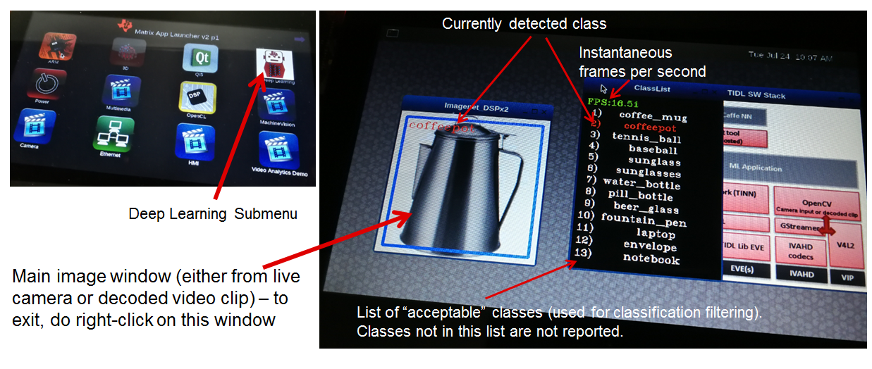
Imagenet classification using Jacinto11 model https://github.com/tidsp/caffe-jacinto-models/tree/caffe-0.17/trained/image_classification/imagenet_jacintonet11v2/sparse, with video input coming from pre-recorded clip. It is decoded in real-time via GStreamer pipeline (involving IVAHD), and sent to OpenCV processing pipeline. Live camera input (default 640x480 resolution), or decoded video clip (320x320 resolution), are scaled down and central-cropped in run-time (using OpenCV API) to 224x224 before sending to TIDL API.
Result of this processing is standard Imagenet classification output (1D vector with 1000 elements). Further, there is provision to define subset of objects expected to be present in video clip or live camera input. This allows additional decision filtering by using list of permitted classes (list is provided as command line argument). Blue bounding rectangle (in main image window) is presented only when valid detection is reported. Class string of last successful is preserved until next detection (so if no object is detected, blue rectangle will disappear, but last class string remains).
Executable invoked from Matrix-GUI is in: /usr/share/ti/tidl/examples/tidl_classification.
root@am57xx-evm:/usr/share/ti/tidl/examples/classification# ./tidl_classification -h
Usage: tidl_classification
  Will run all available networks if tidl is invoked without any arguments.
  Use -c to run a single network.
Optional arguments:
 -c                   Path to the configuration file
 -d <number of DSP cores> Number of DSP cores to use (0 - 2)
 -e <number of EVE cores> Number of EVE cores to use (0 - 2)
 -g <1|2>             Number of layer groups
 -l                   List of label strings (of all classes in model)
 -s                   List of strings with selected classes
 -i                   Video input (for camera:0,1 or video clip)
 -v                   Verbose output during execution
 -h                   Help
Here is an example (invoked from /usr/share/ti/tidl/examples/classification folder), of classification using live camera input - stop at any time with mouse right-click on main image window. In this example two DSP cores only are used, so it could be run on AM5728 device as well:
cd /usr/share/ti/tidl/examples/classification
./tidl_classification -g 1 -d 2 -e 0 -l ./imagenet.txt -s ./classlist.txt -i 1 -c ./stream_config_j11_v2.txt
Another example (invoked from /usr/share/ti/tidl/examples/classification folder), of classification using pre-recorded video input (test2.mp4) - stop at any time with mouse right-click on main image window: Please note that video clip is looped as long as maximum frame count (specified in stream_config_j11_v2.txt) is not exceeded.
cd /usr/share/ti/tidl/examples/classification
./tidl_classification -g 1 -d 2 -e 0 -l ./imagenet.txt -s ./classlist.txt -i ./clips/test2.mp4 -c ./stream_config_j11_v2.txt
On AM5749, we can leverage presence of EVE cores (“-e 2”). Also note that two layergroups are used (indicated with “-g 2”), meaning that two EVEs are involved and only one DSP, with several bottom layers (closest to output) executed on DSP. Also since DSP utilization for 2nd layergroup is low, it can balance workload for two EVEs (running rest of layers):
cd /usr/share/ti/tidl/examples/classification
./tidl_classification -g 2 -d 1 -e 2 -l ./imagenet.txt -s ./classlist.txt -i 1 -c ./stream_config_j11_v2.txt
./tidl_classification -g 2 -d 1 -e 2 -l ./imagenet.txt -s ./classlist.txt -i ./clips/test10.mp4 -c ./stream_config_j11_v2.txt
Slightly higher performance (on AM5749) can be achieved if both DSP and both EVE cores are running concurrently (each core processes one frame independently). Please note that applicability of such approach depends on type of network. If EVE core does processing much faster than the DSP, this is not very useful.
cd /usr/share/ti/tidl/examples/classification
./tidl_classification -g 1 -d 2 -e 2 -l ./imagenet.txt -s ./classlist.txt -i ./clips/test10.mp4 -c ./stream_config_j11_v2.txt
Please note that imagenet.txt is list of all classes (labels) that can be detected by the model specified in configuration file (stream_config_j11_v2.txt). List of filtered (allowed) detections is specified in ./classlist.txt (using subset of strings from imagenet.txt). E.g. currently following subset is used:
- coffee_mug
- coffeepot
- tennis_ball
- baseball
- sunglass
- sunglasses
- water_bottle
- pill_bottle
- beer_glass
- fountain_pen
- laptop
- notebook
Different group of classes using different inputs can be used for user defined testing. In that case, download square images (if aspect is not square, do central cropping first) and place in folder on Linux x86 (that has ImageMagick and ffmpeg installed). Following commands should be executed to create synthetic video clip that can be used in classification example:
# Linux x86 commands to create short video clip out of several static images that are morphed into each other
convert ./*.jpg -delay 500 -morph 300 -scale 320x320 %05d.jpg
ffmpeg -i %05d.jpg -vcodec libx264 -profile:v main -pix_fmt yuv420p -r 15 test.mp4
If video clip is captured or prepared externally (e.g. with the smartphone), object need to be centrally located (in run-time we do resize and central cropping). Then, it should be copied to /usr/share/ti/tidl/examples/classification/clips/ (or just overwrite test1.mp4 in that same folder).
3.15.1.3.2.1. Description of Matrix-GUI classification example
Example is based on “imagenet” and “test” examples, with few additions related to decision filtering and visualization. There are two source files only:
- main.cpp
- Parse command line arguments (ParseArgs) and show help how to use the program (DisplayHelp)
- Initialize configuration (using network model) and executors (DSPs or EVEs), as well as execution objects (frame input and output buffers).
- Create windows with TIDL static image, Decoded clip or Live camera input and window with the list of enabled classes.
- Main processing loop is in RunConfiguration
- Additional functions: tf_postprocess (sort detections and check if top candidate is enabled in the subset) and ShowRegion (if decision is stable for last 3 frames).
- findclasses.cpp
- Function populate_labels(), which reads all the model labels (E.g. 1000 strings for 1000-class imagenet classification model)
- Function populate_selected_items(), which reads and verifies label names (using previous list of valid values), to be used in decision filtering.
3.15.1.3.2.2. Description of Matrix-GUI object detection example
This example is also described in ssd_multibox chapter in TIDL-API docummentation: http://downloads.ti.com/mctools/esd/docs/tidl-api/example.html#ssd Parameeter ‘-p’ defines threshold percentage (0-100 range) for reporting object detections. Lower value is increasing number of false detections, whereas too high value would omit some objects. Participating cores are defined in similar way like in prevous example.
./ssd_multibox -p 40 -d 1 -e 2 -f 1000 -i ./clips/pexels_videos_3623.mp4
Or object detection example using live camera input:
./ssd_multibox -p 40 -d 1 -e 2 -f 1000 -i camera1
Recognized classes are (as defined in http://host.robots.ox.ac.uk/pascal/VOC/voc2012/index.html):
- Person: person
- Animal: bird, cat, cow, dog, horse, sheep
- Vehicle: aeroplane, bicycle, boat, bus, car, motorbike, train
- Indoor: bottle, chair, dining table, potted plant, sofa, tv/monitor
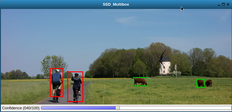
This list can be also found in (target file system): /usr/share/ti/tidl/examples/ssd_multibox/jdetnet_voc_objects.json
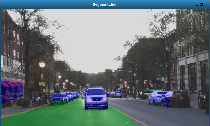
3.15.1.3.2.3. Description of Matrix-GUI image segmentation example
This example shows pixel level image segmentation, also described in TIDL-API docummentation: http://downloads.ti.com/mctools/esd/docs/tidl-api/example.html#segmentation
./segmentation -i ./clips/traffic_pixabay_298.mp4 -f 2000 -w 720
3.15.1.4. Developer’s guide
3.15.1.4.1. Software Stack
Complexity of software is provided for better understanding only. It is expected that the user does programming based on TIDL API only.
In case TIDL uses DSP as accelerator there are three software layers:
- TIDL Library that runs on DSP C66
- OpenCL run-time, which runs on A15, and DSP
- TIDL API host wrapper, user space library
In case TIDL uses EVE as accelerator there are four software layers:
- TIDL Library that runs on EVE
- M4 service layer, acting as proxy between EVE and A15 Linux (considered to be part of OpenCL)
- OpenCL run-time, which runs on A15, but also on M4 (IPU1 which is reserved for TIDL OpenCL monitor role)
- TIDL API host wrapper, user space library
Please note that TIDL API package APIs are identical whether we use DSP or EVE (or both). User only needs to specify accelerator via parameter.
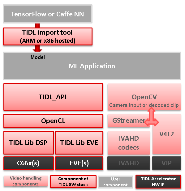
Fig. 3.10 Figure TIDL Software Stack
3.15.1.4.2. Additional public TI resources
Following two Caffe-related repositories (maintained by TI team) provides necessary tools for the training phase. Please use them as primary source of information for training, for TIDL inference software. They include modifications in Caffe source tree to enable higher compute performance (with TIDL inference).
| Repo/URL | Description |
|---|---|
| Caffe-jacinto | fork of NVIDIA/caffe, which in-turn is derived from BVLC/Caffe. The modifications in this fork enable training of sparse, quantized CNN models - resulting in low complexity models that can be used in embedded platforms. Please follow README.md, how to clone, compile and install this version of Caffe. |
| Caffe-jacinto-models | provides example scripts for training sparse models using tidsp/caffe-jacinto. These scripts enable training of sparse CNN models resulting in low complexity models that can be used in embedded platforms. This repository also includes pre-trained models. Additional scripts that can be used to prepare data set and run the training are also available in the scripts folder. |
3.15.1.4.3. Introduction to Programming Model
Public TIDL API interface is described in details at http://downloads.ti.com/mctools/esd/docs/tidl-api/intro.html
In current release it has 3 classes only, allowing use of one or multiple neural network models that can run in parallel on independent EVEs or C66x cores.
Single unit of processing is a tensor (e.g. one image frame, but other inputs are also possible), which is typically processed by single accelerator (EVE or DSP), till completion. But in certain cases it is justified, from performance point of view, to split network layers into two layer groups. Than, we can have one layer group running on EVE and second layer group on DSP. This is done sequentially.
Top layer TIDL API and OpenCL are primarily service software layers (with respect to TIDL software, not NN), i.e. they help in simplifying programming model, IPC mechanism and memory management. Desired features are provided by TIDL Lib which runs in RTOS environment, either on EVE or DSP. This software layer is provided in closed firmware, and used as is, by end user.
3.15.1.4.4. Target file-system
3.15.1.4.4.1. Firmware
OpenCL firmware includes pre-canned DSP TIDL Lib (with hard-coded kernels) and EVE TIDL Lib following Custom Accelerator model. OpenCL firmware is downloaded to DSP and M4/EVE immediately after Linux boot:
- dra7-ipu1-fw.xem4 -> /lib/firmware/dra7-ipu1-fw.xem4.opencl-monitor
- dra7-dsp1-fw.xe66 -> /lib/firmware/dra7-dsp1-fw.xe66.opencl-monitor
- dra7-dsp2-fw.xe66 -> /lib/firmware/dra7-dsp2-fw.xe66.opencl-monitor
3.15.1.4.4.2. User space components
User space TIDL components are included in the Folder /usr/share/ti/tidl and its sub-folders. The sub-folder name and description is as follows:
| Sub folder | Description of content |
|---|---|
| examples | test (file-to-file examples), imagenet classification, image segmentation and SSD multibox examples are here. Matrix GUI example which is based on imagenet one, is in folder tidl_classification. |
| utils | Example configuration files for running the import tool. |
| viewer | Imported model parser and dot graph creator. Input is TIDL model, output is .dot file that can be converted to PNG or PDF format using dot utility (on x86). |
| tidl_api | Source of TIDL API implementation. |
3.15.1.4.5. Input data format
Current release is mainly used with 2D inputs. Most frequent 2D input tensors are color images. Format has to be prepared in same like it was used during model training. Typically, this is following BGR plane interlaced format (common in OpenCV). That means, first 2D array is Blue color plane, next is Green color plane and finally Red color plane.
But, it is perfectly possible to have E.g. two planes on input only: E.g. one plane with Lidar distance measurements and second plane with illumination. This assumes that same format was used during training.
3.15.1.4.6. Output data format
- Image classification
There is 1D vector at the output, one byte per class (log(softmax)). If model has 100 classes, output buffer will 100 bytes long, if model has 1000 classes, output buffer will be 1000 bytes long
- Image segmentation
Output buffer is 2D buffer, typically WxH (Width and Height of input image). Each byte is class index of pixel in input image. Typically count of classes is one or two dozens (but has to be fewer than 255).
- Object detection
Output buffer is a list of tuples including: class index, bounding box (4 parameters) and optionally probability metric.
3.15.1.4.7. Import Process
TIDL import tool converts deep learning models to TI custom network format for efficient execution on TI devices. It supports the following framework/format:
- Caffe
- TensorFlow
- TensorFlow Lite
- ONNX
The import process is done in two steps:
- The first step deals with parsing of model parameters and network topology, and converting them into custom format that TIDL Lib can understand.
- The second step does calibration of dynamic quantization process by finding out ranges of activations for each layer. This is accomplished by invoking simulation (using native C implementation) which estimates initial values important for quantization process. These values are later updated on per frame basis, assuming strong temporal correlation between input frames.
During import process, some operators or layers will be coalesced into one TIDL Layer (e.g. convolution and ReLU layer). This is done to further leverage EVE architecture which allows certain operations for free. Structure of converted (but equivalent) network can be checked using TIDL network viewer.
The import tool (Linux x86 or Arm Linux port) imports the Model and Parameters trained using either Caffe frame work or TensorFlow frame work in PC, or converted from Tensorflow to TensorFlow Lite format, or written in ONNX format. This tool will accept various parameters through import configuration file and generate the Model and Parameter file that the code will be executed using TIDL library across multiple EVE and DSP cores. The import configuration file is available in {TIDL_install_path}/test/testvecs/config/import
There are two pre-built executable binaries for import tool: tidl_model_import.out and eve_test_dl_algo_ref.out. The first one is the main program to run the tool, and the second one is the program to do the calibration and is specified in the configuration file. Both binaries can be referenced by the system path. For Linux x86, linux-devkit/environment-setup needs to be run to setup the path. For AM57xx EVM, they will be in system path after the EVM is setup.
Sample Usage:
tidl_model_import.out ./test/testvecs/config/import/tidl_import_jseg21.txt
3.15.1.4.7.1. Configuration Parameters for Import
The list of import configuration parameters is as below:
| Parameter | Configuration |
|---|---|
| randParams | can be either 0 or 1. Default value is 0. If it is set to 0, the tool will generate the quantization parameters from model, otherwise it will generate random quantization parameters |
| modelType | can be either 0, 1, or 2. Default value is 0. 0 - caffe frame work, 1 - tensor flow frame work, 2 - ONNX frame work. |
| quantizationStyle | can be ‘0’ for fixed quantization by the training framework or ‘1’ for dynamic quantization by. Default value is 1. Currently, only dynamic quantization is supported |
| quantRoundAdd | can take any value from 0 to 100. Default value is 50. quantRoundAdd/100 will be added while rounding to integer |
| numParamBits | can take values from 4 to 12. Default value is 8. This is the number of bits used to quantize the parameters |
| preProcType | can take values from 0 to 6. Default value is 0. Refer to table below for more information about image preprocssing. |
| conv2dKernelType | can be either 0 or 1 for each layer. Set it to 0 to use sparse convolution and set it to 1 to use dense convolution. Default: if this parameter is not set, import tool will automatically set convolution layers with width x height < 64x64 to dense convolution which is optimal for small resolutions, and set other convolution layers to sparse. Note that this parameter must be set for every layer if users choose not to use the default. |
| inElementType | can be either 0 or 1. Default value is 1. Set it to 0 for 8-bit unsigned input or to 1 for 8-bit signed input |
| inQuantFactor | can take values >0. Default value is -1 |
| rawSampleInData | can be either 0 or 1. Default value is 0. Set it to 0, if the input data is encoded, or set it to 1, if the input is RAW data. Note that encoded input is only supported on the target but not on x86 host. |
| numSampleInData | can be > 0. Default value is 1. |
| foldBnInConv2D | can be either 0 or 1. Default value is 1. |
| inWidth | is Width of the input image, it can be >0. |
| inHeight | is Height of the input image, it can be >0 |
| inNumChannels | is input number of channels. It can be from 1 to 1024 |
| sampleInData | is Input data File name |
| tidlStatsTool | is TIDL reference executable for calibration |
| inputNetFile | is Input net file name (From Training frame work) |
| inputParamsFile | is Input Params file name (From Training frame work) |
| outputNetFile | is Output Model net file name, to be updated with stats. |
| outputParamsFile | is Output Params file name |
| layersGroupId | indicates group of layers that needs to be processed on a given CORE. Refer SSD import config for example usage |
| inMean | is a list of mean values for input normalization. inMean = mean*255, where mean are the mean values to normalize input in range [0,1] |
| inScale | is a list of scale values for input normalization. inScale = 1/(std*255), where std are the standard deviations to normalize input in range [0,1] |
Image pre-processing depends on configuration parameters rawSampleInData and preProcType as described below:
| rawSampleInData | preProcType | image pre-processing |
|---|---|---|
| 0 | 0 | Pre-processing for Caffe-Jacinto models:
|
| 0 | 1 | Pre-processing for Caffe models: Resize and crop as preProcType 0, and then subtract pixels by (104, 117, 123) per plane. |
| 0 | 2 | Pre-processing for TensorFlow models:
|
| 0 | 3 | Pre-processing for CIFAR 10:
|
| 0 | 4 | For JDetNet: no pre-processing is performed on the original image. |
| 0 | 5 |
|
| 0 | 6 | Pre-processing for ONNX models: normalize the original image in the range of [0, 255]
|
| 0 | 7-255 | Configuration error. No pre-processing to be done. |
| 0 | 256 | Take inMean and inScale from config file and do the normalization on RAW image:
|
| 0 | >256 | Configuration error. No pre-processing to be done. |
| 1 | N/A | Raw image. No pre-processing to be done, and preProcType is ignored. |
3.15.1.4.7.2. Sample configuration file
Sample configuration files for TIDL import can be found in folder /usr/share/ti/tidl/utils/test/testvecs/config/import. One specific example, tidl_import_j11_v2.txt, is listed below:
# Default - 0
randParams         = 0

# 0: Caffe, 1: TensorFlow, Default - 0
modelType          = 0

# 0: Fixed quantization By tarininng Framework, 1: Dynamic quantization by TIDL, Default - 1
quantizationStyle  = 1

# quantRoundAdd/100 will be added while rounding to integer, Default - 50
quantRoundAdd      = 50

# 0 : 8bit Unsigned, 1 : 8bit Signed Default - 1
inElementType      = 0

rawSampleInData    = 1

# Fold Batch Normalization Layer into TIDL Lib Conv Layer
foldBnInConv2D     = 1

# Weights are quantized into this many bits:
numParamBits       = 12

# Network topology definition file
inputNetFile       = "import/dogs_deploy.prototxt"

# Parameter file
inputParamsFile    = "import/DOGS_iter_34000.caffemodel"

# Translated network stored into two files:
outputNetFile      = "tidl_net_imagenet_jacintonet11v2.bin"
outputParamsFile   = "tidl_param_imagenet_jacintonet11v2.bin"

# Calibration image file
sampleInData = "import/test.raw"

# Reference implementation executable, used in calibration (processes calibration image file)
tidlStatsTool = "eve_test_dl_algo_ref.out"
3.15.1.4.7.3. Import tool traces
During conversion, import tool generates traces reporting detected layers and its parameters (last several columns indicate input tensor dimensions and output tensor dimensions).
Processing config file ./tempDir/qunat_stats_config.txt !
0, TIDL_DataLayer                 ,  0,  -1 ,  1 ,  x ,  x ,  x ,  x ,  x ,  x ,  x ,  x ,  0 ,    0 ,    0 ,    0 ,    0 ,    1 ,    3 ,  224 ,  224 ,
1, TIDL_BatchNormLayer            ,  1,   1 ,  1 ,  0 ,  x ,  x ,  x ,  x ,  x ,  x ,  x ,  1 ,    1 ,    3 ,  224 ,  224 ,    1 ,    3 ,  224 ,  224 ,
2, TIDL_ConvolutionLayer          ,  1,   1 ,  1 ,  1 ,  x ,  x ,  x ,  x ,  x ,  x ,  x ,  2 ,    1 ,    3 ,  224 ,  224 ,    1 ,   32 ,  112 ,  112 ,
3, TIDL_ConvolutionLayer          ,  1,   1 ,  1 ,  2 ,  x ,  x ,  x ,  x ,  x ,  x ,  x ,  3 ,    1 ,   32 ,  112 ,  112 ,    1 ,   32 ,   56 ,   56 ,
4, TIDL_ConvolutionLayer          ,  1,   1 ,  1 ,  3 ,  x ,  x ,  x ,  x ,  x ,  x ,  x ,  4 ,    1 ,   32 ,   56 ,   56 ,    1 ,   64 ,   56 ,   56 ,
5, TIDL_ConvolutionLayer          ,  1,   1 ,  1 ,  4 ,  x ,  x ,  x ,  x ,  x ,  x ,  x ,  5 ,    1 ,   64 ,   56 ,   56 ,    1 ,   64 ,   28 ,   28 ,
6, TIDL_ConvolutionLayer          ,  1,   1 ,  1 ,  5 ,  x ,  x ,  x ,  x ,  x ,  x ,  x ,  6 ,    1 ,   64 ,   28 ,   28 ,    1 ,  128 ,   28 ,   28 ,
7, TIDL_ConvolutionLayer          ,  1,   1 ,  1 ,  6 ,  x ,  x ,  x ,  x ,  x ,  x ,  x ,  7 ,    1 ,  128 ,   28 ,   28 ,    1 ,  128 ,   14 ,   14 ,
8, TIDL_ConvolutionLayer          ,  1,   1 ,  1 ,  7 ,  x ,  x ,  x ,  x ,  x ,  x ,  x ,  8 ,    1 ,  128 ,   14 ,   14 ,    1 ,  256 ,   14 ,   14 ,
9, TIDL_ConvolutionLayer          ,  1,   1 ,  1 ,  8 ,  x ,  x ,  x ,  x ,  x ,  x ,  x ,  9 ,    1 ,  256 ,   14 ,   14 ,    1 ,  256 ,    7 ,    7 ,
10, TIDL_ConvolutionLayer         ,  1,   1 ,  1 ,  9 ,  x ,  x ,  x ,  x ,  x ,  x ,  x , 10 ,    1 ,  256 ,    7 ,    7 ,    1 ,  512 ,    7 ,    7 ,
11, TIDL_ConvolutionLayer         ,  1,   1 ,  1 , 10 ,  x ,  x ,  x ,  x ,  x ,  x ,  x , 11 ,    1 ,  512 ,    7 ,    7 ,    1 ,  512 ,    7 ,    7 ,
12, TIDL_PoolingLayer             ,  1,   1 ,  1 , 11 ,  x ,  x ,  x ,  x ,  x ,  x ,  x , 12 ,    1 ,  512 ,    7 ,    7 ,    1 ,    1 ,    1 ,  512 ,
13, TIDL_InnerProductLayer        ,  1,   1 ,  1 , 12 ,  x ,  x ,  x ,  x ,  x ,  x ,  x , 13 ,    1 ,    1 ,    1 ,  512 ,    1 ,    1 ,    1 ,    9 ,
14, TIDL_SoftMaxLayer             ,  1,   1 ,  1 , 13 ,  x ,  x ,  x ,  x ,  x ,  x ,  x , 14 ,    1 ,    1 ,    1 ,    9 ,    1 ,    1 ,    1 ,    9 ,
15, TIDL_DataLayer                ,  0,   1 , -1 , 14 ,  x ,  x ,  x ,  x ,  x ,  x ,  x ,  0 ,    1 ,    1 ,    1 ,    9 ,    0 ,    0 ,    0 ,    0 ,
Layer ID    ,inBlkWidth  ,inBlkHeight ,inBlkPitch  ,outBlkWidth ,outBlkHeight,outBlkPitch ,numInChs    ,numOutChs   ,numProcInChs,numLclInChs ,numLclOutChs,numProcItrs ,numAccItrs  ,numHorBlock ,numVerBlock ,inBlkChPitch,outBlkChPitc,alignOrNot
  2           72           64           72           32           28           32            3           32            3            1            8            1            3            4            4         4608          896            1
  3           40           30           40           32           28           32            8            8            8            4            8            1            2            4            4         1200          896            1
  4           40           30           40           32           28           32           32           64           32            7            8            1            5            2            2         1200          896            1
  5           40           30           40           32           28           32           16           16           16            7            8            1            3            2            2         1200          896            1
  6           40           30           40           32           28           32           64          128           64            7            8            1           10            1            1         1200          896            1
  7           40           30           40           32           28           32           32           32           32            7            8            1            5            1            1         1200          896            1
  8           24           16           24           16           14           16          128          256          128            8            8            1           16            1            1          384          224            1
  9           24           16           24           16           14           16           64           64           64            8            8            1            8            1            1          384          224            1
 10           24            9           24           16            7           16          256          512          256            8            8            1           32            1            1          216          112            1
 11           24            9           24           16            7           16          128          128          128            8            8            1           16            1            1          216          112            1
  Processing Frame Number : 0
Final output (based on calibration raw image as provided in configuration file), is stored in a file with reserved name: stats_tool_out.bin Size of this file should be identical to count of output classes (in case of classification). E.g. for imagenet 1000 classes, it has to be 1000 bytes big. In addition to final blob, all intermediate results (activations of individual layers), are stored in ./tempDir folder (inside folder where import is invoked). Here is a sample list of files with intermediate activations:
- trace_dump_0_224x224.y <- This very first layer should be identical to the data blob used in desktop Caffe (during validation)
- trace_dump_1_224x224.y
- trace_dump_2_112x112.y
- trace_dump_3_56x56.y
- trace_dump_4_56x56.y
- trace_dump_5_28x28.y
- trace_dump_6_28x28.y
- trace_dump_7_14x14.y
- trace_dump_8_14x14.y
- trace_dump_9_7x7.y
- trace_dump_10_7x7.y
- trace_dump_11_7x7.y
- trace_dump_12_512x1.y
- trace_dump_13_9x1.y
- trace_dump_14_9x1.y
3.15.1.4.7.4. Splitting layers between layers groups
In order to use both DSP and EVE accelerators, it is possible to split the network into two sub-graphs using concept of layergroups. Than one layer group can be executed on EVE and another on DSP. Output of first group (running on EVE) will be used as input for DSP.
This can be accomplished in following way (providing an example for Jacinto11 network):
# Default - 0
randParams         = 0

# 0: Caffe, 1: TensorFlow, Default - 0
modelType          = 0

# 0: Fixed quantization By tarininng Framework, 1: Dynamic quantization by TIDL, Default - 1
quantizationStyle  = 1

# quantRoundAdd/100 will be added while rounding to integer, Default - 50
quantRoundAdd      = 25

numParamBits       = 8
# 0 : 8bit Unsigned, 1 : 8bit Signed Default - 1
inElementType      = 0

inputNetFile       = "../caffe_jacinto_models/trained/image_classification/imagenet_jacintonet11v2/sparse/deploy.prototxt"
inputParamsFile    = "../caffe_jacinto_models/trained/image_classification/imagenet_jacintonet11v2/sparse/imagenet_jacintonet11v2_iter_160000.caffemodel"
outputNetFile      = "./tidl_models/tidl_net_imagenet_jacintonet11v2.bin"
outputParamsFile   = "./tidl_models/tidl_param_imagenet_jacintonet11v2.bin"

sampleInData = "./input/preproc_0_224x224.y"
tidlStatsTool = "./bin/eve_test_dl_algo_ref.out"
layersGroupId    = 0       1       1       1       1       1       1       1       1       1       1       1       2       2       2       0
conv2dKernelType = 0       0       0       0       0       0       0       0       0       0       0       0       1       1       1       1
Input and output layer belong to layer group 0. Layergroup 1 is dispatched to EVE, and layergroup 2 to DSP.
Second row (conv2dKernelType) indicates if convolution is sparse (0) or dense (1). Users may also choose not to set this parameter so that the import tool automatically configures convolution layers to dense or sparse based on kernel sizes.
After conversion, we can visualize the network:
tidl_viewer -p -d ./j11split.dot ./tidl_net_imagenet_jacintonet11v2.bin
dot -Tpdf ./j11split.dot -o ./j11split.pdf
Here is a graph (group 1 is executed on EVE, and group 2 is executed on DSP):
Output of layers group 1 is shared (common) with input buffer of layers group 2 so no extra buffer copy overhead. Due to this buffer allocation, sequential operation of EVE and DSP is necessary.
3.15.1.4.7.5. Calculating theoretical GMACs needed
This can be calculated for up-front for computationally most intensive layers: Convolution Layers and Fully Connected Layers. Each Convolution Layer has certain number of input and output feature maps (2D tensors). Input feature map is convolved with convolution kernel (usually 3x3, but also 5x5, 7x7..). So total number of MACs can be calculated as: Height_input_map x Width_input_map x N_input_maps x N_output_maps x size_of_kernel.
E.g. for 112x112 feature map, with 64 inputs, 64 outputs and 3x3 kernels, we need:
112x112x64x64x3x3 MAC operations = 4624229916 MAC operations
Similarly for fully connected layer, with N_inputs and N_outputs, total number of MAC operations is
E.g. N_inputs = 4096 and N_outputs = 1000,
Fully Connected Layer MAC operations = N_inputs * N_outputs = 4096 * 1000 = 4096000 MAC operations
Obviously Convolution Layer workload is significantly higher.
3.15.1.4.7.6. Mapping to EVE capabilities
Each EVE core can do 16 MAC operation per cycle. Accumulated results are stored in 40-bit accumulator and can be barrel shifted before stored into local memory. Also, EVE can do ReLU operation for free, so frequently, Convolution Layer or Fully Connected Layer is coalesced with ReLU layer.
In order to support these operations wide path to local memory is needed. Concurrently transfers from external DDR memory are performed using dedicated EDMA engines. So, when EVE does convolutions it is always accessing both activations and weights that are already present in high speed local memory.
One or two layers are implemented on EVE local RISC CPU which is used primarily for programming vector engine and EDMA. In these rare cases EVE CPU is used as fully programmable, but slow compute engine. SoftMax layer is implemented using general purpose CPU, and significantly slower than DSP or A15 implementation. As SoftMax layer is terminal layer it is advised to do SoftMax either on A15 (in user space) or using DSP (layergroup2, as implemented in JDetNet examples).
3.15.1.4.8. Verifying TIDL inference result
The TIDL import step runs the inference on PC and the result generates expected output (with caffe or tensorflow inference). If you observe difference at this stage please follow below steps to debug.
- Caffe inference input and TIDL inference input shall match. Import step dumps input of the first layer at “trace_dump_0_*”, make sure that this is same for caffe as well. This is important to verify to avoid mismatch in image pre-processing steps.
- If the input is matching, then dump layer level features from caffe and match with TIDL import traces.
- TIDL trace is in fixed point and can be converted to floating point (using OutQ printed in the import log). Due to quantization the results will not exactly match, but will be similar.
- Check the parameters of the layer where the mismatch is observed.
- Share the input and Parameter with TI for further debug.
We use the statistics collected from the previous process for quantizing the activation dynamically in the current processes. So, results we observe during the process on target will NOT be same (but similar) for same input images compared to import steps. The logic was validated with semantic segmentation application on input video sequence
3.15.1.4.9. Parameters controling dynamic quantization
TIDL Inference process is not completely stateless. Information (activation min, max values) from previously executed inferences are used for quantization process.
- quantMargin is margin added to the average in percentage.
- quantHistoryParam1 weights used for previously processed inference during application boot time (for initial few frames)
- quantHistoryParam2 weights used for previously processed inference during application execution (after initial few frames)
Default settings are:
quantHistoryParam1 = 20;
quantHistoryParam2 = 5;
quantMargin = 0;
Sometimes these parameters need further tuning (via trial and error with similar image sequences).
In order to get the same result in TIDL target like during import step for an image:
quantHistoryParam1 = 0;
quantHistoryParam2 = 0;
quantMargin = 0;
For video sequence, below settings can be also tested:
quantHistoryParam1 = 20;
quantHistoryParam2 = 10;
quantMargin = 20
Quantization parameters are also discussed in API reference
3.15.1.4.10. Importing Tensorflow Models
TIDL supports slim based tensorflow models and only accepts optimized frozen graphs. Following models have been validated:
- MobileNet v1:
- Obtain frozen graph from here
- Optimze the graph using TensorFlow tool:
python "tensorflow\python\tools\optimize_for_inference.py" --input=mobilenet_v1_1.0_224_frozen.pb --output=mobilenet_v1_1.0_224_final.pb --input_names=input --output_names="MobilenetV1/Predictions/Softmax"
- InceptionNet v1 (googleNet):
- Refer to export_inference_graph for generating frozen graph from checkpoint.
- Generate frozen graph from this checkpoint link
- Optimze the graph using TensorFlow tool similarly to MobileNet v1.
3.15.1.4.11. Importing Caffe Models
Caffe models are descibed in two files:
- Network topology definition file in text format
- Network parameter file in binary format
The input layer in network topology file may be defined with various formats, but TIDL import tool only supports the “input_shape” format, for example:
input: "data"
input_shape {
  dim: 1
  dim: 3
  dim: 224
  dim: 224
}
3.15.1.4.12. Viewer tool
Viewer tool does visualization of imported network model. More details available at http://downloads.ti.com/mctools/esd/docs/tidl-api/viewer.html Here is an example command line:
root@am57xx-evm:/usr/share/ti/tidl/examples/test/testvecs/config/tidl_models# tidl_viewer
Usage: tidl_viewer -d <dot file name> <network binary file>
Version: 01.00.00.02.7b65cbb
Options:
-p              Print network layer info
-h              Display this help message


root@am57xx-evm:/usr/share/ti/tidl/examples/test/testvecs/config/tidl_models# tidl_viewer -p -d ./jacinto11.dot ./tidl_net_imagenet_jacintonet11v2.bin
  #  Name                  gId   #i   #o   i0   i1   i2   i3   i4   i5   i6   i7   o   #roi    #ch      h      w   #roi    #ch      h      w
  0, Data                ,  0,  -1 ,  1 ,  x ,  x ,  x ,  x ,  x ,  x ,  x ,  x ,  0 ,    0 ,    0 ,    0 ,    0 ,    1 ,    3 ,  224 ,  224 ,
  1, BatchNorm           ,  1,   1 ,  1 ,  0 ,  x ,  x ,  x ,  x ,  x ,  x ,  x ,  1 ,    1 ,    3 ,  224 ,  224 ,    1 ,    3 ,  224 ,  224 ,
  2, Convolution         ,  1,   1 ,  1 ,  1 ,  x ,  x ,  x ,  x ,  x ,  x ,  x ,  2 ,    1 ,    3 ,  224 ,  224 ,    1 ,   32 ,  112 ,  112 ,
  3, Convolution         ,  1,   1 ,  1 ,  2 ,  x ,  x ,  x ,  x ,  x ,  x ,  x ,  3 ,    1 ,   32 ,  112 ,  112 ,    1 ,   32 ,   56 ,   56 ,
  4, Convolution         ,  1,   1 ,  1 ,  3 ,  x ,  x ,  x ,  x ,  x ,  x ,  x ,  4 ,    1 ,   32 ,   56 ,   56 ,    1 ,   64 ,   56 ,   56 ,
  5, Convolution         ,  1,   1 ,  1 ,  4 ,  x ,  x ,  x ,  x ,  x ,  x ,  x ,  5 ,    1 ,   64 ,   56 ,   56 ,    1 ,   64 ,   28 ,   28 ,
  6, Convolution         ,  1,   1 ,  1 ,  5 ,  x ,  x ,  x ,  x ,  x ,  x ,  x ,  6 ,    1 ,   64 ,   28 ,   28 ,    1 ,  128 ,   28 ,   28 ,
  7, Convolution         ,  1,   1 ,  1 ,  6 ,  x ,  x ,  x ,  x ,  x ,  x ,  x ,  7 ,    1 ,  128 ,   28 ,   28 ,    1 ,  128 ,   14 ,   14 ,
  8, Convolution         ,  1,   1 ,  1 ,  7 ,  x ,  x ,  x ,  x ,  x ,  x ,  x ,  8 ,    1 ,  128 ,   14 ,   14 ,    1 ,  256 ,   14 ,   14 ,
  9, Convolution         ,  1,   1 ,  1 ,  8 ,  x ,  x ,  x ,  x ,  x ,  x ,  x ,  9 ,    1 ,  256 ,   14 ,   14 ,    1 ,  256 ,    7 ,    7 ,
  10, Convolution         ,  1,   1 ,  1 ,  9 ,  x ,  x ,  x ,  x ,  x ,  x ,  x , 10 ,    1 ,  256 ,    7 ,    7 ,    1 ,  512 ,    7 ,    7 ,
  11, Convolution         ,  1,   1 ,  1 , 10 ,  x ,  x ,  x ,  x ,  x ,  x ,  x , 11 ,    1 ,  512 ,    7 ,    7 ,    1 ,  512 ,    7 ,    7 ,
  12, Pooling             ,  1,   1 ,  1 , 11 ,  x ,  x ,  x ,  x ,  x ,  x ,  x , 12 ,    1 ,  512 ,    7 ,    7 ,    1 ,    1 ,    1 ,  512 ,
  13, InnerProduct        ,  1,   1 ,  1 , 12 ,  x ,  x ,  x ,  x ,  x ,  x ,  x , 13 ,    1 ,    1 ,    1 ,  512 ,    1 ,    1 ,    1 , 1000 ,
  14, SoftMax             ,  1,   1 ,  1 , 13 ,  x ,  x ,  x ,  x ,  x ,  x ,  x , 14 ,    1 ,    1 ,    1 , 1000 ,    1 ,    1 ,    1 , 1000 ,
  15, Data                ,  0,   1 , -1 , 14 ,  x ,  x ,  x ,  x ,  x ,  x ,  x ,  0 ,    1 ,    1 ,    1 , 1000 ,    0 ,    0 ,    0 ,    0 ,
Output file is jacinto11.dot, that can be converted to PNG or PDF file on Linux x86, using (E.g.):
dot -Tpdf ./jacinto11.dot -o ./jacinto11.pdf
For networks with two layer groups, viewer generated graph clearly depicts layer group partitioning, typically top layers in EVE and bottom layers in DSP optimal group.
3.15.1.4.13. Simulation Tool
We provide simulation tool both in PLSDK Arm filesystem:
- /usr/bin/eve_test_dl_algo.out, bit-exact emulation (of the target execution)
- /usr/bin/eve_test_dl_algo_ref.out, simulation (faster execution)
and Linux x86 simulation tool (added to the path, after enabling linux-devkit with source environment-setup):
- <PLSDK>/linux-devkit/sysroots/x86_64-arago-linux/usr/bin/eve_test_dl_algo.out, bit-exact emulation (of the target execution)
- <PLSDK>/linux-devkit/sysroots/x86_64-arago-linux/usr/bin/eve_test_dl_algo_ref.out, simulation (faster exeectuion)
For bit-exact simulation, output of simulation tool is expected to be identical to the output of A5749 or AM57xx target. Please use this tool as convenience tool only (E.g. testing model on setup without target EVM).
Simulation tool can be used also to verify converted model accuracy (FP32 vs 8-bit implementation). It can run in parallel on x86 leveraging bigger number of cores (simulation tool is single thread implementation). Due to bit-exact simulation, performance of simulation tool cannot be used to predict target execution time, but it can used to validate model accuracy.
An example of configuration file, which includes specification of frame count to process, input image file (with one or more raw images), numerical format of input image file (signed or unsigned), trace folder and model files:
rawImage    = 1
numFrames   = 1
inData   = "./tmp.raw"
inElementType      = 0
traceDumpBaseName   = "./out/trace_dump_"
outData   = "stats_tool_out.bin"
netBinFile      = "./tidl_net_imagenet_jacintonet11v2.bin"
paramsBinFile   = "./tidl_param_imagenet_jacintonet11v2.bin"
In case multiple images need to be processed, below (or similar) script can be used:
 SRC_DIR=$1

 echo "#########################################################" >  TestResults.log
 echo "Testing in $SRC_DIR" >> TestResults.log
 echo "#########################################################" >> TestResults.log
 for filename in $SRC_DIR/*.png; do
      convert $filename -separate +channel -swap 0,2 -combine -colorspace sRGB ./sample_bgr.png
      convert ./sample_bgr.png  -interlace plane BGR:sample_img_256x256.raw
      ./eve_test_dl_algo.out sim.txt
      echo "$filename Results " >> TestResults.log
      hd stats_tool_out.bin | tee -a TestResults.log
done
Simulation tool ./eve_test_dl_algo.out is invoked with single command line argument:
./eve_test_dl_algo.out sim.txt
Simulation configuration file includes list of network modesl to execute, in this case only one: tild_config_j11.txt List is termined with: “0 ”:
1 ./tidl_config_j11_v2.txt
0
Sample confiuguration file used by simulation tool (tidl_config_j11_v2.txt):
rawImage    = 1
numFrames   = 1
preProcType  = 0
inData   = "./sample_img_256x256.raw"
traceDumpBaseName   = "./out/trace_dump_"
outData   = "stats_tool_out.bin"
updateNetWithStats   = 0
netBinFile      = "./tidl_net_model.bin"
paramsBinFile   = "./tidl_param_model.bin"
Results for all images in SRC_DIR will be directed to TestResults.log, and can be tested against Caffe-Jacinto desktop execution.
3.15.1.4.14. Summary of model porting steps
- After model creation using desktop framework (Caffe or TF), it is ncessary to verify accuracy of the model (using inference on desktop framework: Caffe/Caffe-Jacinto or TensorFlow).
- Import the final model (in case of Caffe-Jacinto, at the end of “sparse” phase) using above import procedure
- Verify accuracy (using smaller test data set than the one used in first step) using simulation tool. - Drop in accuracy (vs first step) should not be big (few percents).
- Test the network on the target, using TIDL API based program and imported model.
3.15.1.5. Compatibility of trained model formats
Below versions of frameworks or runtimes have been used for testing the TIDL import procedure and execution of imported models in TIDL runtime. Below information should be used in addition to constraints related to operator availability in TIDL library. More recent versions of formats might be also supported, but not guaranteed.
- Caffe: v1.0
- Tensorflow: v1.12
- Tensorflow Lite: v1.15
- ONNX runtime: v1.4
3.15.1.6. Training
Existing Caffe and TF-Slim models can be imported as long as layers are supported and parameter constraints are met. But, typically these models include dense weight matrices. In order to leverage some benefits of TIDL Lib, and gain 3x-4x performance improvement (for Convolution Layers), it is necessary to repeat the training process using caffe-jacinto caffe fork, available at https://github.com/tidsp/caffe-jacinto Highest contribution to Convolution Neural Networks compute load comes from Convolution Layers (often in 80-90% range), hence special attention is paid to optimize Convolution Layer processing.
Data set preparation should follow standard Caffe approach, typically creating LMDB files. After that training is done in 3 steps:
- Initial training (typically with L2 regularization), creating dense model.
This phase is actually usual training procedure applied on desktop. At the end of this phase, it is necessary to verify accuracy of the model. Weight tensors are dense so performance target may not be hit but following steps can improve the performance. If accuracy is not sufficient, it is not advisible to proceed with further steps (they won’t improve accuracy - actually small drop in accruacy of 1-2% is expected). Instead, modify training parameters or enhance data set, and repeat the training, until accuracy target is met.
- L1 regularization
This step is necessary to (opposite to L2) favor certain weight values at the expense of others, and make larger portion weights smaller. Remaining weights would behave like feature extractors (required for next step).
- Sparse (“sparsification”)
By gradual adjustment of weight threshold (from smaller to higher) sparsification target is tested at each step (E.g. 70% or 80%). This procedure eliminates small weights, leaving bigger contributors only. Please note that this applies to Convolution Layers only.
- Define acceptable criteria for sparsification based on accuracy drop
Due to conversion from FP32 representation to 8-12 bit representation of weights (and 8-bit activations), acceptable accuracy drop should be within 1-2% range (depending on model), E.g. if classification accuracy for Caffe-Jacinto desktop model is 70% (using model after initial phase), we should not see lower accuracy for sparsified and quantized model below 68%.
3.15.1.6.1. Example of training procedure
- Setup for data set collection of specific smaller objects.
Apart from many publicly available image data sets, it is frequently the case that new data set need to be collected for specific use case. E.g. in industrial environment, is typically more predictable and often it is possible to ensure controlled environment with good illumination. For pick-and-place applications, set of objects that can appear in camera field-of-view is not infinite, but rather confined to few or few dozens classes. Using turn-table and photo booth with good illumination allows quick data set collection.
- Data set collection using AM57xx
Data set images can be recorded by external camera device, or even using Camera Daughter card (of AM57xx). Suggested recorded format is H264, that offers good quality and can be efficiently decoded using GStreamer pipeline. It can last 15-20 seconds only (rotation period of turn-table). With slower fps (10-15fps), this provides 200-300 frames. Procedure can be repeated by changing distance and elevation (3-4 times), so total image count can be up to 2000-3000 frames per class. This can limit single class data collection time to 5-10min.
- Post-processing
Video clips should be copied to Linux x86 for offline post-processing. FFMPEG package allows easy splitting of video clips into individual images. Since recording is made against uniform background, it is also possible to apply automated labeling procedure. Additional data set enhancements can be made using image augmentation scripts, easily increasing count of images 10-20x.
- Prepare LMDB files for the training
Please refer to available scripts in github.com/tidsp/caffe-jacinto-models/scripts
- Do training from scratch or do transfer learning (fine-tuning)
Frequently, it is good to start training using initial weights created with generic data set (like ImageNet). Bottom layers act like feature extractors, and only top 1 or few layers need to be fine tuned using data set that we just collected (as described in previous sets). In case of Jacinto11, good starting point is model created after “Initial” phase. We will need to repeat initial phase, but now using new data set, and using same layer names for those layers that we want to pre-load with earlier model. Further, training can be tuned by reducing base_lr (in train.prototxt), and increasing lr for top one or few layers. In this way bottom layers will be changed superficially, but top layers will adapt as necessary. Matrix-GUI toy dog breeds classification example is created in this way. Imagenet trained Jacinto11 model is fine-tuned using custom data set of toy dogs. Recrodings of toy dogs standing on turn table, were captured using AM5749 camera. They were later split into individual images and augmented for offline training.
3.15.1.6.2. Where does the benefit of sparsification come from?
- Initially Deep Learning networks were implemented using Single Precision floating-point arithmetic’s (FP32). During last few years, more research has been done regarding quantization impact and reduced accuracy of arithmetic operations. In many cases, 8-bits, or even less (down to 2-4 bits) are considered sufficient for correct operation. This is explained with huge number of parameters (weights) that all contribute to operation accuracy. In case of DSP and EVE inference implementation, weights (controlled by parameter in import tool configuration file) can be quantized with 8-12 bit accuracy. Activation layer outputs (neuron output) are stored in memory with 8-bit accuracy (single byte). Accumulation is done with 40-bit accuracy, but final output is right-shifted before single byte is stored into memory. Right shift count is determined dynamically, uniquely for each layer and once per frame. More details can be found in http://openaccess.thecvf.com/content_cvpr_2017_workshops/w4/papers/Mathew_Sparse_Quantized_Full_CVPR_2017_paper.pdf
- Additional optimization (described in above article) is based on sparsification of Convolution Layer weights. Individual weights are forced to zero during training. This is achieved during “L1 regularization” phase (enforcing fewer bigger weights at the expense of others) and “Sparse” when small weights are clamped to zero. We can specify desired training target (E.g. 70% or 80% of all weights to be zero). During inference, computation is reorganized so that multiplication with single weight parameter is done across all input values. If weight is zero multiplication against all input data (for that input channel) is skipped. All computation are done using pre-loaded blocks into local L2 memory (using “shadow” EDMA transfers).
3.15.1.7. Performance data
3.15.1.7.1. Computation performance of verified networks
- Results in below table are collected FOR SINGLE CORE execution (EVE or DSP), with AM5729. EVE running at 650MHz and DSP running at 750MHz (CCS Setup, single core).
| Network topology | ROI size | MMAC (million MAC) | Sparsity (%) | EVE using sparse model | EVE using dense model | DSP using sparse model | DSP using dense model | EVE + DSP (optimal model) |
|---|---|---|---|---|---|---|---|---|
| MobileNetV1 | 224x224x3 | 567.70 | 1.42 | 155ms | 717.11ms | |||
| MobileNetV2 | 224x224x3 | 146ms | 409ms | 78.1ms | ||||
| SqueezeNet1.1 | 227x227x3 | 390.8 | 1.46 | 180ms | 433.73ms | |||
| InceptionNetV1 | 224x224x3 | 1497.37 | 2.48 | 362ms | 1454.91ms | |||
| JacintoNet11_v2 | 224x224x3 | 405.81 | 73.15 | 92.23ms | 181ms | 115.91ms | 370.64ms | 58.16 |
| JSegNet21 | 1024x512x3 | 8506.5 | 76.47 | 299.ms | 1005.49ms | 1101.12ms | 3825.95ms | |
| JDetNet | 768x320x3 | 2191.44 | 61.84 | 158.60ms |
- Models for TI defined topologies: JacintoNet11, JSeg21 and JDetNet can be obtained from: https://github.com/tidsp/caffe-jacinto-models/tree/caffe-0.17/trained
- Sparsity provided in above table is average sparsity across all convolution layers.
- Optimal Model – with optimal placement of layers between EVE and DSP (certain NN layers run faster on DSP, like SoftMax; ARP32 in EVE emulates float operation in software, so this can be rather slow).
3.15.1.8. Multi core performance (EVE and DSP cores only)
- Results in below table are collected FOR MULTI CORE execution, with AM5729 device and using various sets of EVE and DSP cores.
- Test script used for collecting below statistics can be found in target file system: /usr/share/ti/tidl/examples/mcbench/ (e.g.: source ./scripts/all_5749.sh)
| Devices | AM5728,AM5749,AM5729 | AM5749,AM5729 | AM5749, AM5729 | AM5729 | AM5729 | ||
|---|---|---|---|---|---|---|---|
| Network topology | Mode | ROI size | 2xDSP (1 layers group) | 2xEVE (1 layers group) | Optimal: 2xEVE+1xDSP (2 layers groups) | 4xEVE (1 layers group) | Optimal: 4xEVE+1xDSP (2 layers groups) |
| MobileNetV1 | Classif. | 224x224x3 | 2.69 roi/s | 13.7 roi/s | 21.57 roi/s | 25.05 roi/s | 39.1 roi/s |
| MobileNetV2 | Classif. | 224x224x3 | 4.88 roi/s | 13.5 roi/s | 24.27 roi/s | 24.8 roi/s | 42.2 roi/s |
| SqueezeNet1.1 | Classif. | 224x224x3 | 4.46 roi/s | 11 roi/s | 14.7 roi/s | 21.64 roi/s | 32.4 roi/s |
| InceptionNetV1 | Classif. | 224x224x3 | 1.34 roi/s | 5.46 roi/s | 6.62 roi/s | 10.73 roi/s | 12.93 roi/s |
| JacintoNet11_v2, dense | Classif. | 224x224x3 | 5.32 roi/s | 10.2 roi/s | 13.6 roi/s | 20.2 roi/s | 26.8 roi/s |
| JacintoNet11_v2, sparse | Classif. | 224x224x3 | 16.9 roi/s | 19.1 roi/s | 34.7 roi/s | 36.1 roi/s | 64.6 roi/s |
| JSegNet21, dense | Segment. | 1024x512x3 | 1.76 roi/s | 0.47 roi/s | 3.37 roi/s | ||
| JSegNet21, sparse | Segment. | 1024x512x3 | 2.43 roi/s | 6.32 roi/s | 11.8 roi/s | ||
| JDetNet, sparse | Obj.Det. | 768x320x3 | 12.98 roi/s | 22.56 roi/s | |||
- Optimal Model (as discussed in previous paragraph) typically requires last 2-3 layers to be executed on DSP, especially if they involve FP32 calculations (like SoftMax).
- Layers groups can be defined in runtime using 2 layers group configuration: first layers group is executed on EVE and second on DSP. TIDL-API takes care of execution pipelining.
- Properly setting configuration for conv2dkernelype parameter is very important for execution performance of layers with feature map size smaller than 64x64: dense type is mandatory for layers with small feature maps (dense is ‘1’, sparese is ‘0’). This parameter is applicable on per layer basis (multiple values are expected - as many as there are layers).
- In upcoming releases conv2dkernelytype setting will be done automatically during import process.
- From release PLSDK 5.1, default EVE speed is increased from 535MHz to 650MHz.
3.15.1.8.1. Accuracy of selected networks
Below tables are copied here for convenience, from https://github.com/tidsp/caffe-jacinto-models documents.
- Image classification : Top-1 classification accuracy indicates probability that ground truth is ranked highest. Top-5 classification accuracy indicates probability that ground truth is among top-5 ranking candidates.
| Configuration-Dataset Imagenet (1000 classes) | Top-1 accuracy |
|---|---|
| JacintoNet11 non-sparse | 60.9% |
| JacintoNet11 layerwise threshold sparse (80%) | 57.3% |
| JacintoNet11 channelwise threshold sparse (80%) | 59.7% |
- Image segmentation : Mean Intersection over Union is ratio between True Positives and sum of True Positives, False Negatives and False Positives
| Configuration-Dataset Cityscapes (5-classes) | Pixel accuracy | Mean IOU |
|---|---|---|
| Initial L2 regularized training | 96.20% | 83.23% |
| L1 regularized training | 96.32% | 83.94% |
| Sparse fine tuned (~80% zero coefficients) | 96.11% | 82.85% |
| Sparse (80%), Quantized (8-bit dynamic fixed point) | 95.91% | 82.15% |
- Object Detection : Validation accuracy can be in classification accuracy or mean average precision (mAP). Please note change in accuracy between “Initial” (dense) and “Sparse” model (performance boost can be 2x-4x):
| Configuration-Dataset VOC0712 | mAP |
|---|---|
| Initial L2 regularized training | 68.66% |
| L1 regularized fine tuning | 68.07% |
| Sparse fine tuned (~61% zero coefficients) | 65.77% |
3.15.1.9. Troubleshooting
- Application with TIDL doesn’t run at all
- Verify that CMEM is active and running:
- cat /proc/cmem
- lsmod | grep “cmem”
- Default CMEM size is not sufficient for devices with more than 2 EVEs (make ~56-64MB available per EVE).
- Validate OpenCL stack is running
Upon Linux boot, OpenCL firmwares are downloaded to DSP and EVE. As OpenCL monitor for IPU1 (which controls EVEs) is new addition, here is expected trace: Enter following command on target: cat /sys/kernel/debug/remoteproc/remoteproc0/trace0 Following output is expected, indicating number of available EVE accelerators (below AM5729 trace indicates 4 EVEs):
[0][      0.000] 17 Resource entries at 0x3000
[0][      0.000] [t=0x000aa3b3] xdc.runtime.Main: 4 EVEs Available
[0][      0.000] [t=0x000e54bf] xdc.runtime.Main: Creating msg queue...
[0][      0.000] [t=0x000fb885] xdc.runtime.Main: OCL:EVEProxy:MsgQ ready
[0][      0.000] [t=0x0010a1a1] xdc.runtime.Main: Heap for EVE ready
[0][      0.000] [t=0x00116903] xdc.runtime.Main: Booting EVEs...
[0][      0.000] [t=0x00abf9a9] xdc.runtime.Main: Starting BIOS...
[0][      0.000] registering rpmsg-proto:rpmsg-proto service on 61 with HOST
[0][      0.000] [t=0x00b23903] xdc.runtime.Main: Attaching to EVEs...
[0][      0.007] [t=0x00bdf757] xdc.runtime.Main: EVE1 attached
[0][      0.010] [t=0x00c7eff5] xdc.runtime.Main: EVE2 attached
[0][      0.013] [t=0x00d1b41d] xdc.runtime.Main: EVE3 attached
[0][      0.016] [t=0x00db9675] xdc.runtime.Main: EVE4 attached
[0][      0.016] [t=0x00dc967f] xdc.runtime.Main: Opening MsgQ on EVEs...
[0][      1.017] [t=0x013b958a] xdc.runtime.Main: OCL:EVE1:MsgQ opened
[0][      2.019] [t=0x019ae01a] xdc.runtime.Main: OCL:EVE2:MsgQ opened
[0][      3.022] [t=0x01fa62bf] xdc.runtime.Main: OCL:EVE3:MsgQ opened
[0][      4.026] [t=0x025a4a1f] xdc.runtime.Main: OCL:EVE4:MsgQ opened
[0][      4.026] [t=0x025b4143] xdc.runtime.Main: Pre-allocating msgs to EVEs...
[0][      4.027] [t=0x0260edc5] xdc.runtime.Main: Done OpenCL runtime initialization. Waiting for messages...
- TIDL import tool doesn’t give enough information
The import tool will fail to import a model if it is not in supported format (Caffe/TensorFlow/ONNX). E.g. following report can be seen if format is not recognized:
$ ./tidl_model_import.out ./modelInput/tidl_import_mymodel.txt
TF Model File : ./modelInput/mymodel
Num of Layer Detected :   0
Total Giga Macs : 0.0000

Processing config file ./tempDir/qunat_stats_config.txt !
  0, TIDL_DataLayer                ,  0,   0 ,  0 ,  x ,  x ,  x ,  x ,  x ,  x ,  x ,  x ,  0 ,    0 ,    0 ,    0 ,    0 ,    0 ,    0 ,    0 ,    0 ,

Processing Frame Number : 0

End of config list found !
- Target execution is different from desktop Caffe execution
To debug this, we can use simulation tool as it is bit-exact with EVE or DSP execution. Traces that are generated by simulation tool can be visually compared against data blobs that are saved after desktop Caffe inference. If all the rest is correct, it is worth comparing intermediate results. Please keep in mind that numerical equivalence between Caffe desktop computation (using single precision FP32) and target computation (using 8-bit activations, and 8-12 bit weights) are not expected. Still features maps (of intermediate layers) are supposed to be rather similar. If something is significantly different, please try to change number of bits for weights, or repeat import processing with more representative image. Problems of this sort should be rarely encountered.
- Following error is seen in runtime
... inc/executor.h:199: T* tidl::malloc_ddr(size_t) [with T = char; size_t = unsigned int]: Assertion `val != nullptr' failed.
This means that previous run failed to de-allocate CMEM memory. Reboot is one option, restarting ti-mctd deamon is another option.
- Caffe import crashes with error message
[libprotobuf FATAL <protobuf path>/protobuf/repeated_field.h:1478] CHECK failed: (index) < (current_size_):
terminate called after throwing an instance of 'google::protobuf::FatalException'
what():  CHECK failed: (index) < (current_size_):
Aborted (core dumped)
This is usually caused by unsupported Caffe input layer format. For more details, refer to Importing Caffe Models.
- TensorFlow import failed with error “Could not find the requested input Data:”
This is likely due to unoptimized frozen graphs. Refer Importing Tensorflow Models for more details.