5.3. Application Demos
5.3.1. Dual Camera
Dual camera demo
Below diagram illustrates the video data processing flow of dual camera demo.
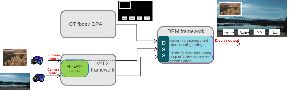
Dual camera example demo demonstrates following-
- Video capture using V4L2 interface from up to two cameras.
- QT QWidget based drawing of user interface using linuxfb plugin. linuxfb is fbdev based software drawn QPA.
- Hardware accelerated scaling of input video from primary camera to display resolution using DSS IP.
- Hardware accelerated scaling of input video from secondary camera (if connected) to lower resolution using DSS IP.
- Hardware accelerated overlaying of two video planes and graphics plane using DSS IP.
- Scaling of two video planes and overlaying with graphics plane happens on the fly in single pass inside DSS IP using DRM atomic APIs.
- Snapshot of the screen using JPEG compression running on ARM. The captured images are stored in filesystem under /usr/share/camera-images/ folder
- The camera and display driver shares video buffer using dmabuf protocol. Capture driver writes captured content to a buffer which is directly read by the display driver without copying the content locally to another buffer (zero copy involved).
- The application also demonstrates allocating the buffer from either omap_bo (from omapdrm) memory pool or from cmem buffer pool. The option to pick omap_bo or cmem memory pool is provided runtime using cmd line.
- If the application has need to do some CPU based processing on captured buffer, then it is recommended to allocate the buffer using CMEM buffer pool. The reason being omap_bo memory pool doesn’t support cache read operation. Due to this any CPU operation involving video buffer read will be 10x to 15x slower. CMEM pool supports cache operation and hence CPU operations on capture video buffer are fast.
- The application runs in nullDRM/full screen mode (no windows manager like wayland/x11) and the linuxfb QPA runs in fbdev mode. This gives applicationfull control of DRM resource DSS to control and display the video planes.
Instructions to run dual camera demo
- Since the application need control of DRM resource (DSS) and there can be only one master, make sure that the wayland/weston is not running.
#/etc/init.d/weston stop
- Run the dual camera application
#dual-camera -platform linuxfb <0/1>
- When last argument is set as 0, capture and display driver allocates memory from omap_bo pool.
- When it is set to 1, the buffers are allocated from CMEM pool.
5.3.2. Video Analytics
Overview
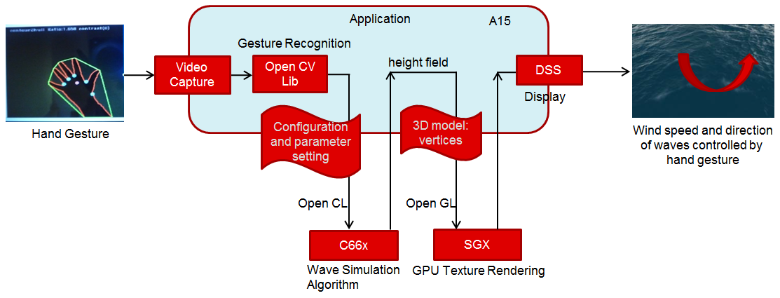
The Video Analytics demo shipped with the Processor SDK Linux for AM57xx showcases how a Linux Application running on Cortex A-15 cluster can take advantage of C66x DSP, 3D SGX hardware acceleration blocks to process a real-time camera input feed and render the processed output on display - all using open programming paradigms such as OpenCV, OpenCL, OpenGL, and Qt and standard Linux drivers for capture/display.
A hand gesture is detected using morphological operators from OpenCV library. The gesture is used to control a parameter (wind speed) used in physical simulation of water waves. Result of simulation is visualized in real-time via 3D rendering of water surface. The hardware IP blocks, such as IVAHD, M4 cores, are not utilized for this demo.
Setup
In order to re-create the demo, user would need a standard AM572x GP EVM and Processor SDK Linux package. The demo is integrated into the Matrix GUI and can be launched by touching the “Video Analytics” icon on the LCD. The sources to the demo are packaged in the Processor SDK Linux Installer, under “example-applications” folder and can be compiled using the SDK’s top-level Makefile
Building Blocks
- Camera Capture: The camera module on AM572x GP EVM acquires color frames of 640x480 resolution. The images are received by the OpenCV framework using camera capture class, that depends on the standard V4L2 Linux driver (/dev/video1).
- Gesture Recognition: The first 30 frames captured are used to estimate the background, and later subtracted to extract the hand contour, using erode and dilute operations available in the OpenCV Library. Analysis of largest contour is performed to find convex hulls. Hand gesture classification is based on ratio of outer and inner contour. Several discrete values are sent to wave simulation algorithm.
- Wave Simulation: Wave simulation is done in two stages: calculation of initial (t=0)) Phillips spectrum followed by spectrum updates per each time instant. Height map is generated in both steps using 2D IFFT (of spectrum). The Gesture inputs are used to vary the wind direction for wave simulation
- Graphics Rendering: Finally, 2D vertex grid is generated with the above height map. Fragment rendering uses user-defined texture and height dependent coloring.
- Display: The displayed content includes - Camera feed, overlayed with the contour detection, and the generated water surface
Block diagram
Demo Internals
Programming Paradigm
- Code running on A15 Linux platform is written in C++ and links with QT5, OpenCV and OpenCL host side libraries.
- Code running on DSP C66x is written in OpenCL C
- Code running on GPU is written in GLSL.
- Standard V4L2 Linux driver is used for camera capture
- The demo uses OpenCV 3.1, OpenCL 1.2, OpenGL ES 2.0/GLSL and QT 5.5
OpenCV (running on ARM A15s)
Video analytics functionality includes simple algorithm to extract contours of hand, and detect how widely opened the hand is. A parameter which indicates ratio between convex hull and contours is used to control physical simulation of waves.This is an output argument converted to wind speed, in 2.5-10 ms range (4 discrete values). Initially image background is estimated (for 30 frames) using MOG2 (Mixture Of Gaussians), standard OpenCV algorithm. Later, the background is subtracted from camera frames, before morphological operations: erode and dilute are performed.Next two steps include contour detection (which is also presented in camera view window) and convex hull estimation. Ratio between outer and inner contour indicates (in 1.1-1.8 range) can be correlated with number of fingers and how widely are they spread. If they are more widely spread, parameter is converted to higher wind speed and waves become higher.
OpenCL (running on ARM A15s + C66x)
Wave surface simulation is based on generation of Phillips (2D) spectrum followed by 2D IFFT (256x256). Both operations are executed by OpenCL offload to single DSP core. Many details on this algorithm can be found in graphics.ucsd.edu/courses/rendering/2005/jdewall/tessendorf.pdf. This stage is controlled by wave speed (output of gesture detection algorithm) using fixed wind direction (an idea for improvement: wind direction can be controlled using hand gesture).
Height map in form of 256x256 float matrix is generated on output and used by OpenGL based vertex renderer (performed in next step). Wave surface simulation consists of two steps:
- initial setup defining starting conditions (wind speed and wind direction are used as input in this stage only)
- update of wave surface height map (Phillips spectrum modification generated at t=0, along time axe and 2D IFFT for each time step).
OpenGL ES (running on ARM A15s + GPU/SGX)
FLOW: 256x256 float height map matrix + fixed texture -> OpenGL ES based algorithm -> rendered frame buffers
OpenGL ES is a subset of Open GL for desktop devices. Important difference (for this project) is requirement to use vertex buffers and only triangle strips. Also Qt provides wrapper functions (QOpenGL functions) created with intention to hide differences between different OpenGL versions and also to slightly simplify programming. On the downside, it involves Qt specific syntax (not far from original OpenGL ES functions). Height Map data (256x256, but sub-sampled by 4x4, hence 64x64 vertices) received from previous stage, are rendered specific coloring and user supplied JPEG image. Fragment shader does mixing of texture and color derived from interpolated height giving more natural visualization. Currently lighting effects are not used (Implementing this can significantly improve the quality of rendering).
QT 5 (running on ARM A15)
FLOW: user input (mouse and keyboard) -> QT application -> windowing system and control of above threads
Directory Structure
The functionality is organized as shows in the files/description below.
| file name | description | |
| 1 | CameraConnectDialog.cpp/CameraConnectDialog.h | |
| 2 | CameraGrab.cpp/CameraGrab.h | Auxilliary camera frame acquisition functions to achieve full FPS |
| 3 | CameraView.cpp/CameraView.h | Major class instantiated after connecting to camera. This class creates processing thread, wavesimulation thread and also instantiates wave display (3D graphics) widget. |
| 4 | CaptureThread.cpp/CaptureThread.h | Input (camera) frame buffering. |
| 5 | FrameLabel.cpp/FrameLabel.h | |
| 6 | GeometryEngine.cpp/GeometryEngine.h | Height map mash creation, vertex updates |
| 7 | Gesture.cpp/Gesture.h | Hand gesture (OpenCV) detection algorith, |
| 8 | ImageProcessingSettingsDialog.cpp/ImageProcessingSettingsDialog.h | Settings of parameters used by image processing algorithms. |
| 9 | main.cpp | main function |
| 10 | MainWindow.cpp/MainWindow.h | |
| 11 | MatToQImage.cpp/MatToQImage.h | Conversion from OpenCV Mat object to QT QImage object |
| 12 | ProcessingThread.cpp/ProcessingThread.h | Main processing thread, frame rate dynamics, invokes variois image processing algorithms |
| 13 | SharedImageBuffer.cpp/SharedImageBuffer.h | |
| 14 | WaveDisplayWidget.cpp/WaveDisplayWidget.h | Wave surface 3D rendering (invokes methods from GeometryEngine.cpp) |
| 15 | WaveSimulationThread.cpp/WaveSimulationThread.h | Wave surface physical simulation thread - host side of OpenCL dispatch. |
| 16 | Buffers.h | |
| 17 | Structures.h | |
| 18 | Config.h | |
| 19 | phillips.cl | DSP OpenCL phillips spectrum generation kernels and 2D IFFT kernel (invoking dsplib.ae66 optimized 1D FFT). After compilation (by clocl) phillips.dsp_h is generated, and included in WaveSimulationThread.cpp (ocl kernels are compiled and downloaded in this thread, before run-time operation is started). |
| 20 | vshader.glsl | Vertex shader (gets projection matrix, position and texture position as input arguments; generates texture coordinate and height for fragment shader |
| 21 | fshader.glsl | Fragment shader doing linear interpolation of textures and mixing texture with height dependent color, and adds ambient light |
| 22 | shaders.qrc | Specify shader filenames |
| 23 | textures.qrc | Specify texture file (2D block which is linearly interpolated in fragment shader, using position arguments provided by vertex shader) |
| 24 | qt-opencv-multithreaded.pro | Top level QT make file: phi |
| 25 | ImageProcessingSettingsDialog.ui | User interface definition file for modification of algorithm parameters. |
| 26 | CameraView.ui | Camera view user interface definition file - right click mouse action brings up image processing algorithm selection |
| 27 | CameraConnectDialog.ui | |
| 28 | MainWindow.ui |
Performance
The hand gesture detection/wave surface simulation/wave surface rendering demo pipeline runs at 18-20 fps. For other algorithms (e.g. smoothing, canny) the pipeline runs at 33-35 fps.
Licensing
The demo code is provided under BSD/MIT License
FAQ/Known Issues
- Brighter lighting conditions are necessary for noise-free camera input, to allow good contour detection. In poor lighting conditions, there would be false or no detection.
- OpenCV 3.1 version shows low FPS rate for Camera Capture. Hence, a custom solution based on direct V4L2 ioctl() calls is adopted (cameraGrab.cpp file) to boost the FPS
5.3.3. DLP 3D Scanner
This demo demonstrates an embedded 3D scanner based on the structured light principle, with am57xx. More details can be found at https://www.ti.com/tool/tidep0076
5.3.4. People Tracking
This demo demonstrates the capability of people tracking and detection with TI’s ToF (Time-of-Flight) sensor. More details can be found at https://www.ti.com/lit/pdf/tidud06
5.3.5. Barcode Reader
Introduction
Detecting 1D and 2D barcodes on an image, and decoding those barcodes are important use cases for the Machine-Vision. Processor SDK Linux has integrated the following open source components, and examples to demonstrate both of these features.
- Barcode detection: OpenCV
- Barcode Decoder/Reader: Zbar Library
OpenCV includes python wrapper to allow quick and easy prototyping. It also includes support for OpenCL offload on devices with C66 DSP core (currently OpenCV T-API cannot be used with python wrapper).
Zbar Barcode Decoder/Reader
Recipes for zbar barcode reader have been added to build the zbar library and test binary. Zbar is standalone library, which does not depend on OpenCV. Current release is not accelerated via OpenCL dispatch (obvious candidates are zbar_scan_y() and calc_tresh() functions consuming >50% of CPU resources).
Command to run zbar test binary:
barcode_zbar [barcode_image_name]
Barcode Region Of Interest (ROI) Detection with OpenCV and Python
Detecting Barcodes in Images using Python and OpenCV provides python scripts which run with OpenCV 2.4.x. For use with Process SDK Linux which has OpenCV 3.1, modifications have been made to the original python scripts so that they can run with OpenCV 3.1. Below please find the modified python scripts detect_barcode.py.
# import the necessary packages
import numpy as np
import argparse
import cv2

# construct the argument parse and parse the arguments
ap = argparse.ArgumentParser()
ap.add_argument("-i", "--image", required = True, help = "path to the image file")
args = vars(ap.parse_args())

# load the image and convert it to grayscale
image = cv2.imread(args["image"])
gray = cv2.cvtColor(image, cv2.COLOR_BGR2GRAY)

# compute the Scharr gradient magnitude representation of the images
# in both the x and y direction
gradX = cv2.Sobel(gray, ddepth = cv2.CV_32F, dx = 1, dy = 0, ksize = -1)
gradY = cv2.Sobel(gray, ddepth = cv2.CV_32F, dx = 0, dy = 1, ksize = -1)

# subtract the y-gradient from the x-gradient
gradient = cv2.subtract(gradX, gradY)
gradient = cv2.convertScaleAbs(gradient)

# blur and threshold the image
blurred = cv2.blur(gradient, (9, 9))
(_, thresh) = cv2.threshold(blurred, 225, 255, cv2.THRESH_BINARY)

# construct a closing kernel and apply it to the thresholded image
kernel = cv2.getStructuringElement(cv2.MORPH_RECT, (21, 7))
closed = cv2.morphologyEx(thresh, cv2.MORPH_CLOSE, kernel)

# perform a series of erosions and dilations
closed = cv2.erode(closed, None, iterations = 4)
closed = cv2.dilate(closed, None, iterations = 4)

# find the contours in the thresholded image, then sort the contours
# by their area, keeping only the largest one
(_, cnts, _) = cv2.findContours(closed.copy(), cv2.RETR_EXTERNAL,cv2.CHAIN_APPROX_SIMPLE)
c = sorted(cnts, key = cv2.contourArea, reverse = True)[0]

# compute the rotated bounding box of the largest contour
rect = cv2.minAreaRect(c)
box = np.int0(cv2.boxPoints(rect))

# draw a bounding box arounded the detected barcode and display the
# image
cv2.drawContours(image, [box], -1, (0, 255, 0), 3)
cv2.imshow("Image", image)
cv2.waitKey(0)
python detect_barcode.py --image [barcode_image_name]
Barcode Region Of Interest (ROI) Detection with OpenCV and CPP implementation
Current version of OpenCV (3.1) Python wrapper does not support T-API which is needed for OpenCL dispatch. So Processor SDK Linux is including the same algorithm implemented in CPP (https://git.ti.com/apps/barcode-roi-detection), which can be executed on ARM platform only, or with DSP acceleration. CPP example includes more options for various types of input and output, and run-time control of OpenCL dispatch.
This example allows multiple command line options:
- Using static image (JPG or PNG) as input
- Live display or static image output (JPG or PNG)
- Use OpenCL offload or not
Target filesystem includes detect_barcode in “/usr/bin”, and test vector in “/usr/share/ti/image” folder. Again, after successful detection image with barcode in green bounding box is displayed or written to output file. Below are various use cases of detect_barcode.
- Static image input, no opencl dispatch, live display: detect_barcode sample_barcode.jpg 0 1
- Static image input, opencl ON, live display: detect_barcode sample_barcode.jpg 1 1
- Static image input, opencl ON, file output: detect_barcode sample_barcode.jpg 1 image_det.png
Majority of workload is in following lines:
ocl::setUseOpenCL(ocl_acc_flag);  /* Turn ON or OFF OpenCL dispatch  */

cvtColor(im_rgb,im_gray,CV_RGB2GRAY);
im_gray.copyTo(img_gray);

Sobel( img_gray, gradX, CV_16S, 1, 0, -1, 1, 0, BORDER_DEFAULT ); /* Input is 8-bit unsigned, output is 16-bit signed */
Sobel( img_gray, gradY, CV_16S, 0, 1, -1, 1, 0, BORDER_DEFAULT ); /* Input is 8-bit unsigned, output is 16-bit signed */
subtract(gradX, gradY, gradient);
convertScaleAbs(gradient, abs_gradient);

// blur and threshold the image
//GaussianBlur( abs_gradient, blurredImg, Size(7,7), 0, 0, BORDER_DEFAULT );
GaussianBlur( abs_gradient, blurredImg, Size(3,3), 0, 0, BORDER_DEFAULT ); /* 3x3 kernel */
threshold(blurredImg, threshImg, 225, 255, THRESH_BINARY);

Mat elementKernel = getStructuringElement( MORPH_RECT, Size( 2*10+1, 2*3+1 ), Point(10, 3));
ocl::setUseOpenCL(false); /* Turn OFF OpenCL dispatch */
morphologyEx( threshImg, closedImg, MORPH_CLOSE, elementKernel );

ocl::setUseOpenCL(ocl_acc_flag);   /* Turn ON or OFF OpenCL dispatch  */
erode(closedImg, img_final, UMat(), Point(-1, -1), 4); /* erode, 4 iterations */
dilate(img_final, img_ocl, UMat(), Point(-1, -1), 4);  /* dilate, 4 iteration */
ocl::setUseOpenCL(false); /* Turn OFF OpenCL dispatch */
Not all OpenCV kernels can be dispatched to DSP via OpenCL. Please refer to OpenCV#OpenCL_C_C66_DSP_kernels for the list of kernels which are currently DSP accelerated.
In order to use OpenCL dispatch, it is necessary to:
- Enable OpenCL use (by setting environment variables, and invoking ocl::setUseOpenCL(ocl_acc_flag))
- Use T-API: e.g. replace Mat types with UMat types
5.3.6. EVSE Demos
This demo showcases Human Machine Interface (HMI) for Electric Vehicle Supply Equipment(EVSE) Charging Stations. More details can be found at https://www.ti.com/tool/TIDEP-0087
5.3.7. Protection Relay Demo
Matrix UI provides out of box demo to showcase Human Machine Interface (HMI) for Protection Relays. More details can be found at https://www.ti.com/tool/TIDEP-0102
5.3.8. mmWave Gesture Controlled HMI
This demo showcases gesture controlled HMI, where the mmWave sensor detects presence and classifies natural hand gestures, and sends them to the Sitara processor to drive the Qt GUI display. More details can be found at https://www.ti.com/tool/TIDEP-01013.
5.3.9. Qt5 Thermostat HMI Demo
Qt-based Thermostat HMI demo
The morphing of devices like the basic thermostat into a breed of power smart thermostats has shown how the appliances in residences today must adapt, re-imagine and, in some cases, reinvent their role in the connected home of the future or risk being left behind. Thermostats in particular have come a long way since they were first created. There was a time when the mechanical dial thermostat was the only option. It was simple and intuitive to operate because what you saw was what you got. The user simply set the temperature and walked away. Unfortunately, it was not efficient. Energy and money could be wasted since its settings would only change when someone manually turned the dial to a new temperature. Modern thermostats provide a much richer Graphical Interface, with several features. Processor SDK now includes a Qt5 based thermostat with the following key features - that should easily enable customers to use as a starting point for further innovation.
- Display three-day weather forecast, daily temperature range for the selected city from openweathermap.org
- Display and adjust room temperature
- Pop-up menu to select city, temperature format and set network proxy
- Weekly temperature schedule
- Away Energy saving mode
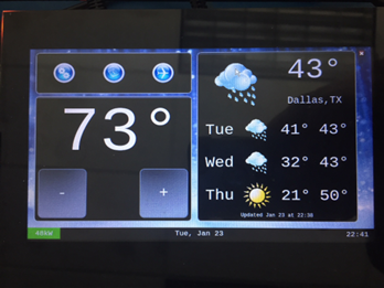
Fig. 5.1 Figure1: three-day weather forecast
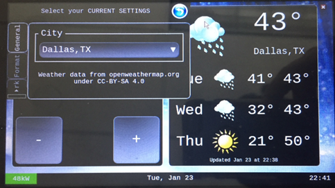
Fig. 5.2 Figure2: Select City for weather forecasts
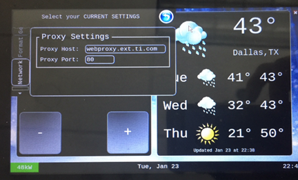
Fig. 5.3 Figure3: Set Proxy for Internet connectivity
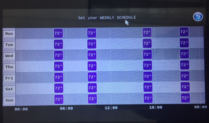
Fig. 5.4 Figure4: Weekly temperature schedule
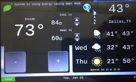
Fig. 5.5 Figure5: Inside temperature, Away energy saving settings
The demo is hosted at https://git.ti.com/apps/thermostat-demo, and also the sources are located at
<SDK-install-dir>/example-applications/qt-tstat-2.0/
The code can be compiled, installed using top-level SDK Makefile
make qt-tstat-clean
make qt-tstat
make qt-tstat-install
5.3.10. Optical Flow with OpenVX
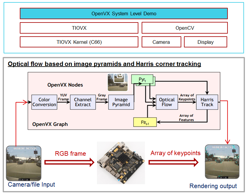
5.3.10.1. OpenVX Example Block Diagram
OpenVx tutorial example demontrates the optical flow based on image pyramids and Harris corner tracking. It builds upon TIOVX, and utilizes OpenCV for reading the input (from file or camera) and rending the output for display. Input frame from OpenCV invokes OpenVX graph, and the processing is done once per input frame. OpenVX defines the graph topology and all configuration details. All resources are allocated and initialzied before processing.
5.3.10.2. Run OpenVx Tutorial Example
The binary for OpenVX tutorial example is located at /usr/bin/tiovx-opticalflow. It is a statically linked Linux application running on Arm.
Before running the tutorial example, download the test clip and copy it to file system (e.g. ~/tiovx). Then, execute the commands below to load OpenVx firmware and run the optical flow example.
reload-dsp-fw.sh tiovx                                       # load openvx firmware and restart dsps
tiovx-opticalflow /home/root/tiovx/PETS09-S1-L1-View001.avi  # Run tutorial example
Screen capture after running the optical flow example:
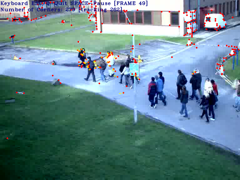
Logs:
root@am57xx-evm:~# tiovx-opticalflow /home/root/PETS09-S1-L1-View001.avi
 VX_ZONE_INIT:Enabled
 VX_ZONE_ERROR:Enabled
 VX_ZONE_WARNING:Enabled
VSPRINTF_DBG:SYSTEM NOTIFY_INIT: starting
VSPRINTF_DBG: SYSTEM: IPC: Notify init in progress !!!

VSPRINTF_DBG:[0] DUMP ALL PROCS[3]=DSP1
VSPRINTF_DBG:[1] DUMP ALL PROCS[4]=DSP2
VSPRINTF_DBG:Next rx queue to open:QUE_RX_HOST

VSPRINTF_DBG:Just created MsgQue
VSPRINTF_DBG:Created RX task
VSPRINTF_DBG:Next tx queue to open:QUE_RX_DSP1, procId=3
VSPRINTF_DBG:Next tx queue to open:QUE_RX_DSP2, procId=4
VSPRINTF_DBG:Dump all TX queues: procId=3 name=QUE_RX_DSP1 queId=262272, msgSize=68, heapId=0
VSPRINTF_DBG:Dump all TX queues: procId=4 name=QUE_RX_DSP2 queId=196736, msgSize=68, heapId=0
VSPRINTF_DBG:SYSTEM: IPC: SentCfgMsg, procId=3 queuId=262272
VSPRINTF_DBG:SYSTEM: IPC: SentCfgMsg, procId=4 queuId=196736
VSPRINTF_DBG: SYSTEM: IPC: Notify init DONE !!!

VSPRINTF_DBG:>>>> ipcNotifyInit returned: 0

VSPRINTF_DBG:SYSTEM NOTIFY_INIT: done
OK: FILE /home/root/PETS09-S1-L1-View001.avi 768x480
init done
Using Wayland-EGL
wlpvr: PVR Services Initialised
LOG: [ status = -1 ] Hello there!
Run the optical flow example with camera input:
reload-dsp-fw.sh tiovx        # load openvx firmware and restart dsps
tiovx-opticalflow             # Run tutorial example with camera input
Logs:
root@am57xx-evm:~# tiovx-opticalflow
 VX_ZONE_INIT:Enabled
 VX_ZONE_ERROR:Enabled
 VX_ZONE_WARNING:Enabled
VSPRINTF_DBG:SYSTEM NOTIFY_INIT: starting
VSPRINTF_DBG: SYSTEM: IPC: Notify init in progress !!!

VSPRINTF_DBG:[0] DUMP ALL PROCS[3]=DSP1
VSPRINTF_DBG:[1] DUMP ALL PROCS[4]=DSP2
VSPRINTF_DBG:Next rx queue to open:QUE_RX_HOST

VSPRINTF_DBG:Just created MsgQue
VSPRINTF_DBG:Created RX task
VSPRINTF_DBG:Next tx queue to open:QUE_RX_DSP1, procId=3
VSPRINTF_DBG:Next tx queue to open:QUE_RX_DSP2, procId=4
VSPRINTF_DBG:Dump all TX queues: procId=3 name=QUE_RX_DSP1 queId=262272, msgSize=68, heapId=0
VSPRINTF_DBG:Dump all TX queues: procId=4 name=QUE_RX_DSP2 queId=196736, msgSize=68, heapId=0
VSPRINTF_DBG:SYSTEM: IPC: SentCfgMsg, procId=3 queuId=262272
VSPRINTF_DBG:SYSTEM: IPC: SentCfgMsg, procId=4 queuId=196736
VSPRINTF_DBG: SYSTEM: IPC: Notify init DONE !!!

VSPRINTF_DBG:>>>> ipcNotifyInit returned: 0

VSPRINTF_DBG:SYSTEM NOTIFY_INIT: done
OK: CAMERA#1 640x480
init done
Using Wayland-EGL
wlpvr: PVR Services Initialised
LOG: [ status = -1 ] Hello there!
After finishing running the OpenVX tutorial example, switch the firmware back to the default for OpenCL:
reload-dsp-fw.sh opencl # load opencl firmware and restart dsps
5.3.11. ROS and Radar
5.3.11.1. Introduction
The ROS is meta-ros running on top of Linux. It is a collection of software libraries and packages to help you write robotic applications. Both mobile platforms and static manipulators can leverage wide colelction of open-source drivers and tools. ROS framework is mainly based on publisher-subscriber model, and in some cases server-client mode.
It is frequently the case that ROS based applications require sensors enabling interaction with the environment. Various types of sensors can be used: cameras, ultrasound, time-of-flight RGBD cameras, lidars, ...
In case of 3D sensors, typical output is point cloud. Consumer of this information (e.g. for navigation) is decoupled from point cloud producer since format is well defined. Due to modular nature of ROS it is easy to replace one sensor with the other as long as format of information (in this case point cloud) is the same.
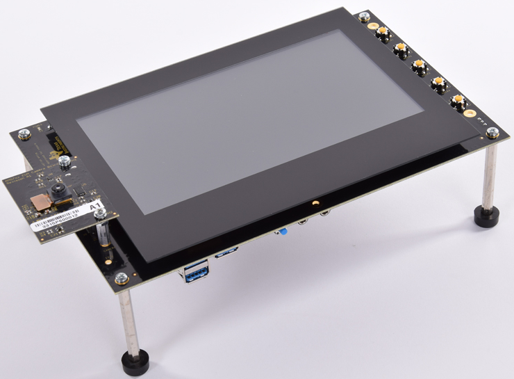
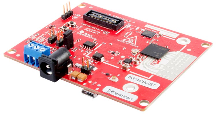
An important type of 3D sensor, especially suited for outdoor use cases is mmWave radar (77-81GHz). For this demo IWR/AWR-1443 or 1642 EVM is needed. It is connected to Sitara device over USB connection creating virtual UART.
Optionally to make this platform movable, Kobuki mobile base can be added. Sitara EVM and Radar EVM would be attached to Kobuki, and Sitara EVM running ROS would control Kobuki movement via USB connection. Please note that mobile base is not essentail for verification of ROS on Sitara plus Radar EVM operation.
It is desirable to have Ubuntu Linux box (typically Linux PC desktop or laptop) with Ubuntu 14.04LTS and ROS indigo installed (please note that ROS Indigo is natively supported in Ubuntu 14.04).
5.3.11.2. HW Setup
- USB to microUSB cable (connecting USB connector on Sitara side with microUSB connector on Radar EVM
- [optional] Kobuki mobile base (as used by Turtlebot2), http://kobuki.yujinrobot.com/

Fig. 5.6 Kobuki mobile base with Sitara, Radar EVMs and monitoring Ubuntu Linux box (PC desktop or laptop)
Compatibility
The ti_mmwave_rospkg ROS driver package on Sitara is tested with Processor Linux SDK which includes meta-ros layer, indigo, (from https://github.com/bmwcarit/meta-ros).
For visualization we use ROS indigo distro on Ubuntu Linux box, preffered for compatibility reasons. Run the commands below to install ROS indigo on Ubuntu Linux box. More details can be found from https://wiki.ros.org/indigo/Installation/Ubuntu.
sudo sh -c 'echo "deb http://packages.ros.org/ros/ubuntu trusty main" > /etc/apt/sources.list.d/ros-latest.list'
wget https://raw.githubusercontent.com/ros/rosdistro/master/ros.key -O - | sudo apt-key add -
sudo apt-get update
sudo apt-get install ros-indigo-desktop-full
For this demo, IWR EVM requires mmWave SDK firmware. If different firmware is used on Radar EVM, please follow procedure using UniFlash tool to install mmWave SDK.
5.3.11.3. ROS configuration verification
ROS is part of PLSDK 4.3 target filesystem, including mmWave ROS driver, so no additional installation steps are required. ROS is installed in /opt/ros/indigo folder. Only setting up configuration related to specific IP address of target EVM, and Ubuntu Linux box host IP address is needed. ROS is distributed meta-ros, with single ROS host acting as a broker for all internode transcations. It runs roscore node and in this case roscore is executed on Sitara. Ubuntu Linux box will only run ROS RViz node since RViz requires OpenGL desktop support (Sitara only supports OpenGL ES 2.0).
Note
If visualization using RViz is not needed, Ubuntu Linux box is not necessary for this demo (except to start multiple SSH terminals).
Reconfigure PLSDK for Python3
PLSDK includes ROS packages from meta-ros layer, compiled with Python3 support (build/conf/local.conf : ROS_USE_PYTHON3 = “yes”) As PLSDK default python setting is Python 2.7, filesystem update is required for ROS tests to run:
root@am57xx-evm:/usr/bin# ln -sf python3 python.python
root@am57xx-evm:/usr/bin# ln -sf python3-config python-config.python
5.3.11.4. ROS between distributed nodes (Sitara and Ubuntu Linux box)
1st SSH terminal, to Sitara EVM
Modify /opt/ros/indigo/setup.bash
export ROS_ROOT=/opt/ros/indigo
export PATH=$PATH:/opt/ros/indigo/bin
export LD_LIBRARY_PATH=/opt/ros/indigo/lib
export PYTHONPATH=/usr/lib/python3.5/site-packages:/opt/ros/indigo/lib/python3.5/site-packages
export ROS_MASTER_URI=http://$SITARA_IP_ADDR:11311
export ROS_IP=$SITARA_IP_ADDR
export CMAKE_PREFIX_PATH=/opt/ros/indigo
export ROS_PACKAGE_PATH=/opt/ros/indigo/share
touch /opt/ros/indigo/.catkin
Then, execute
source /opt/ros/indigo/setup.bash
roscore
2nd SSH terminal, to Sitara EVM
source /opt/ros/indigo/setup.bash
rosrun roscpp_tutorials talker
You will see log similar to following:
....[ INFO] [1516637959.231163685]: hello world 5295
[ INFO] [1516637959.331163994]: hello world 5296
[ INFO] [1516637959.431165605]: hello world 5297
[ INFO] [1516637959.531161359]: hello world 5298
[ INFO] [1516637959.631162807]: hello world 5299
[ INFO] [1516637959.731166207]: hello world 5300
[ INFO] [1516637959.831215641]: hello world 5301
[ INFO] [1516637959.931165361]: hello world 5302
[ INFO] [1516637960.031165019]: hello world 5303
[ INFO] [1516637960.131164027]: hello world 5304
3rd SSH terminal, to Linux BOX (Optional)
export ROS_MASTER_URI=http://$SITARA_IP_ADDR:11311
export ROS_IP=$LINUXBOX_IP_ADDR
source /opt/ros/indigo/setup.bash
rosrun roscpp_tutorials listener
You will see log similar to following:
...
data: hello world 5338
---
data: hello world 5339
---
data: hello world 5340
---
data: hello world 5341
---
data: hello world 5342
---
data: hello world 5343
---
data: hello world 5344
5.3.11.5. mmWave ROS node on Sitara and RViz on Ubuntu Linux box
1st SSH terminal, to Sitara EVM
Start roscore, only if it is not already started
source /opt/ros/indigo/setup.bash roscore
2nd SSH terminal, to Sitara EVM
source /opt/ros/indigo/setup.bash
roslaunch  ti_mmwave_rospkg rviz_1443_3d.launch

Change "rviz_1443_3d.launch to "rviz_1642_2d.launch", based on Radar EVM type (1443 or 1642).
If Kobuki mobile is available, use the command below instead:
roslaunch ti_mmwave_rospkg plsdk_rviz_1443_3d.launch
Sample log is included:
source /opt/ros/indigo/setup.bash
roslaunch ti_mmwave_rospkg plsdk_rviz_1443_3d.launch

... logging to /home/root/.ros/log/97dfe396-2711-11e8-bd4a-a0f6fdc25c34/roslaunch-am57xx-evm-7487.log
Checking log directory for disk usage. This may take awhile.
Press Ctrl-C to interrupt
Done checking log file disk usage. Usage is <1GB.

started roslaunch server http://192.168.0.222:35481/

SUMMARY
========

PARAMETERS
 * /fake_localization/use_map_topic: True
 * /mmWave_Manager/command_port: /dev/ttyACM0
 * /mmWave_Manager/command_rate: 115200
 * /mmWave_Manager/data_port: /dev/ttyACM1
 * /mmWave_Manager/data_rate: 921600
 * /mmWave_Manager/max_allowed_azimuth_angle_deg: 90
 * /mmWave_Manager/max_allowed_elevation_angle_deg: 90
 * /rosdistro: b'<unknown>\n'
 * /rosversion: b'1.11.21\n'

NODES
  /
    fake_localization (fake_localization/fake_localization)
    mmWaveQuickConfig (ti_mmwave_rospkg/mmWaveQuickConfig)
    mmWave_Manager (ti_mmwave_rospkg/ti_mmwave_rospkg)
    octomap_server (octomap_server/octomap_server_node)
    static_tf_map_to_base_radar_link (tf/static_transform_publisher)
    static_tf_map_to_odom (tf/static_transform_publisher)

ROS_MASTER_URI=http://192.168.0.222:11311

core service [/rosout] found
process[mmWave_Manager-1]: started with pid [7505]
process[mmWaveQuickConfig-2]: started with pid [7506]
process[static_tf_map_to_odom-3]: started with pid [7507]
process[static_tf_map_to_base_radar_link-4]: started with pid [7508]
[ INFO] [1520981858.224293205]: mmWaveQuickConfig: Configuring mmWave device using config file: /opt/ros/indigo/share/ti_mmwave_rospkg/cfg/1443_3d.cfg
process[octomap_server-5]: started with pid [7509]
process[fake_localization-6]: started with pid [7517]
[ INFO] [1520981858.367713151]: waitForService: Service [/mmWaveCommSrv/mmWaveCLI] has not been advertised, waiting...
[ INFO] [1520981858.436009564]: Initializing nodelet with 2 worker threads.
[ INFO] [1520981858.480256524]: mmWaveCommSrv: command_port = /dev/ttyACM0
[ INFO] [1520981858.480407967]: mmWaveCommSrv: command_rate = 115200
[ INFO] [1520981858.497923263]: waitForService: Service [/mmWaveCommSrv/mmWaveCLI] is now available.
[ INFO] [1520981858.498667137]: mmWaveQuickConfig: Ignored blank or comment line: '% ***************************************************************'
[ INFO] [1520981858.499059815]: mmWaveQuickConfig: Ignored blank or comment line: '% Created for SDK ver:01.01'
[ INFO] [1520981858.499462577]: mmWaveQuickConfig: Ignored blank or comment line: '% Created using Visualizer ver:1.1.0.1'
[ INFO] [1520981858.505357942]: mmWaveQuickConfig: Ignored blank or comment line: '% Frequency:77'
[ INFO] [1520981858.506164932]: mmWaveQuickConfig: Ignored blank or comment line: '% Platform:xWR14xx'
[ INFO] [1520981858.506843089]: mmWaveQuickConfig: Ignored blank or comment line: '% Scene Classifier:best_range_res'
[ INFO] [1520981858.507514414]: mmWaveQuickConfig: Ignored blank or comment line: '% Azimuth Resolution(deg):15 + Elevation'
[ INFO] [1520981858.508289684]: mmWaveQuickConfig: Ignored blank or comment line: '% Range Resolution(m):0.044'
[ INFO] [1520981858.508999398]: mmWaveQuickConfig: Ignored blank or comment line: '% Maximum unambiguous Range(m):9.01'
[ INFO] [1520981858.509816310]: mmWaveQuickConfig: Ignored blank or comment line: '% Maximum Radial Velocity(m/s):5.06'
[ INFO] [1520981858.510520982]: mmWaveQuickConfig: Ignored blank or comment line: '% Radial velocity resolution(m/s):0.64'
[ INFO] [1520981858.518476684]: mmWaveQuickConfig: Ignored blank or comment line: '% Frame Duration(msec):33.333'
[ INFO] [1520981858.519262364]: mmWaveQuickConfig: Ignored blank or comment line: '% Range Detection Threshold (dB):9'
[ INFO] [1520981858.519957764]: mmWaveQuickConfig: Ignored blank or comment line: '% Range Peak Grouping:disabled'
[ INFO] [1520981858.520157681]: mmWaveDataHdl: data_port = /dev/ttyACM1
[ INFO] [1520981858.520252841]: mmWaveDataHdl: data_rate = 921600
[ INFO] [1520981858.520315142]: mmWaveDataHdl: max_allowed_elevation_angle_deg = 90
[ INFO] [1520981858.520375654]: mmWaveDataHdl: max_allowed_azimuth_angle_deg = 90
[ INFO] [1520981858.520943849]: mmWaveQuickConfig: Ignored blank or comment line: '% Doppler Peak Grouping:disabled'
[ INFO] [1520981858.521671945]: mmWaveQuickConfig: Ignored blank or comment line: '% Static clutter removal:disabled'
[ INFO] [1520981858.522412729]: mmWaveQuickConfig: Ignored blank or comment line: '% ***************************************************************'
[ INFO] [1520981858.523396537]: mmWaveQuickConfig: Sending command: 'sensorStop'
[ INFO] [1520981858.533674630]: mmWaveCommSrv: Sending command to sensor: 'sensorStop'
[ INFO] [1520981858.536083724]: DataUARTHandler Read Thread: Port is open
[ INFO] [1520981858.548926257]: mmWaveCommSrv: Received response from sensor: 'sensorStop
Done
mmwDemo:/>'
[ INFO] [1520981858.550875817]: mmWaveQuickConfig: Command successful (mmWave sensor responded with 'Done')
[ INFO] [1520981858.551745758]: mmWaveQuickConfig: Sending command: 'flushCfg'
[ INFO] [1520981858.559882020]: mmWaveCommSrv: Sending command to sensor: 'flushCfg'
[ INFO] [1520981858.562726084]: mmWaveCommSrv: Received response from sensor: 'flushCfg
Done
mmwDemo:/>'
[ INFO] [1520981858.564378289]: mmWaveQuickConfig: Command successful (mmWave sensor responded with 'Done')
[ INFO] [1520981858.565240748]: mmWaveQuickConfig: Sending command: 'dfeDataOutputMode 1'
[ INFO] [1520981858.573026625]: mmWaveCommSrv: Sending command to sensor: 'dfeDataOutputMode 1'
[ INFO] [1520981858.576915985]: mmWaveCommSrv: Received response from sensor: 'dfeDataOutputMode 1
Done
mmwDemo:/>'
...
mmwDemo:/>'
[ INFO] [1520981858.776118886]: mmWaveQuickConfig: Command successful (mmWave sensor responded with 'Done')
[ INFO] [1520981858.776938726]: mmWaveQuickConfig: Sending command: 'compRangeBiasAndRxChanPhase 0.0 1 0 1 0 1 0 1 0 1 0 1 0 1 0 1 0 1 0 1 0 1 0 1 0'
[ INFO] [1520981858.782736816]: mmWaveCommSrv: Sending command to sensor: 'compRangeBiasAndRxChanPhase 0.0 1 0 1 0 1 0 1 0 1 0 1 0 1 0 1 0 1 0 1 0 1 0 1 0'
[ INFO] [1520981858.792102024]: mmWaveCommSrv: Received response from sensor: 'compRangeBiasAndRxChanPhase 0.0 1 0 1 0 1 0 1 0 1 0 1 0 1 0 1 0 1 0 1 0 1 0 1 0
Done
mmwDemo:/>'
[ INFO] [1520981858.793846462]: mmWaveQuickConfig: Command successful (mmWave sensor responded with 'Done')
[ INFO] [1520981858.794657355]: mmWaveQuickConfig: Sending command: 'measureRangeBiasAndRxChanPhase 0 1.5 0.2'
[ INFO] [1520981858.800233568]: mmWaveCommSrv: Sending command to sensor: 'measureRangeBiasAndRxChanPhase 0 1.5 0.2'
[ INFO] [1520981858.806256139]: mmWaveCommSrv: Received response from sensor: 'measureRangeBiasAndRxChanPhase 0 1.5 0.2
Done
mmwDemo:/>'
[ INFO] [1520981858.807890614]: mmWaveQuickConfig: Command successful (mmWave sensor responded with 'Done')
[ INFO] [1520981858.808687680]: mmWaveQuickConfig: Sending command: 'sensorStart'
[ INFO] [1520981858.814534734]: mmWaveCommSrv: Sending command to sensor: 'sensorStart'
[ INFO] [1520981858.822598283]: mmWaveCommSrv: Received response from sensor: 'sensorStart
Done
mmwDemo:/>'
[ INFO] [1520981858.824211611]: mmWaveQuickConfig: Command successful (mmWave sensor responded with 'Done')
[ INFO] [1520981858.824545077]: mmWaveQuickConfig: mmWaveQuickConfig will now terminate. Done configuring mmWave device using config file: /opt/ros/indigo/share/ti_mmwave_rospkg/cfg/1443_3d.cfg
[mmWaveQuickConfig-2] process has finished cleanly
3rd SSH terminal, to Sitara EVM
Bring up all ROS components for communicting and controlling Kobuki
source /opt/ros/indigo/setup.bash
roslaunch kobuki_node minimal.launch
4th SSH terminal, to Sitara EVM
Start Kobuki teleop console (remotely control Kobuki movement using keyboard)
source /opt/ros/indigo/setup.bash
roslaunch kobuki_keyop safe_keyop.launch

        Operating kobuki from keyboard:
        Forward/back arrows : linear velocity incr/decr.
        Right/left arrows : angular velocity incr/decr.
        Spacebar : reset linear/angular velocities.
        d : disable motors.
        e : enable motors.
        q : quit.
5th SSH terminal, to Ubuntu Linux box
First, install ROS Indigo distribution on Ubuntu Linux box if it has not been done before.
Setup ROS variables on Ubuntu Linux box (to enable communication with ROS host on Sitara) then start RViz
export ROS_MASTER_URI=http://$SITARA_IP_ADDR:11311 (IP address of Sitara EVM, modify as needed)
export ROS_IP=$LINUX_BOX_IP_ADDR (IP address of Ubuntu Linux box, modify as needed)
source /opt/ros/indigo/setup.bash

rosrun rviz rviz
Alternatively, in order to get Kobuki avatar on the screen, install kobuki_description on Ubuntu Linux box and start RViz by launching view_model from kobuki_description.
git clone https://github.com/yujinrobot/kobuki
cd kobuki
cp -r kobuki_description /opt/ros/indigo/share
roslaunch kobuki_description view_model.launch
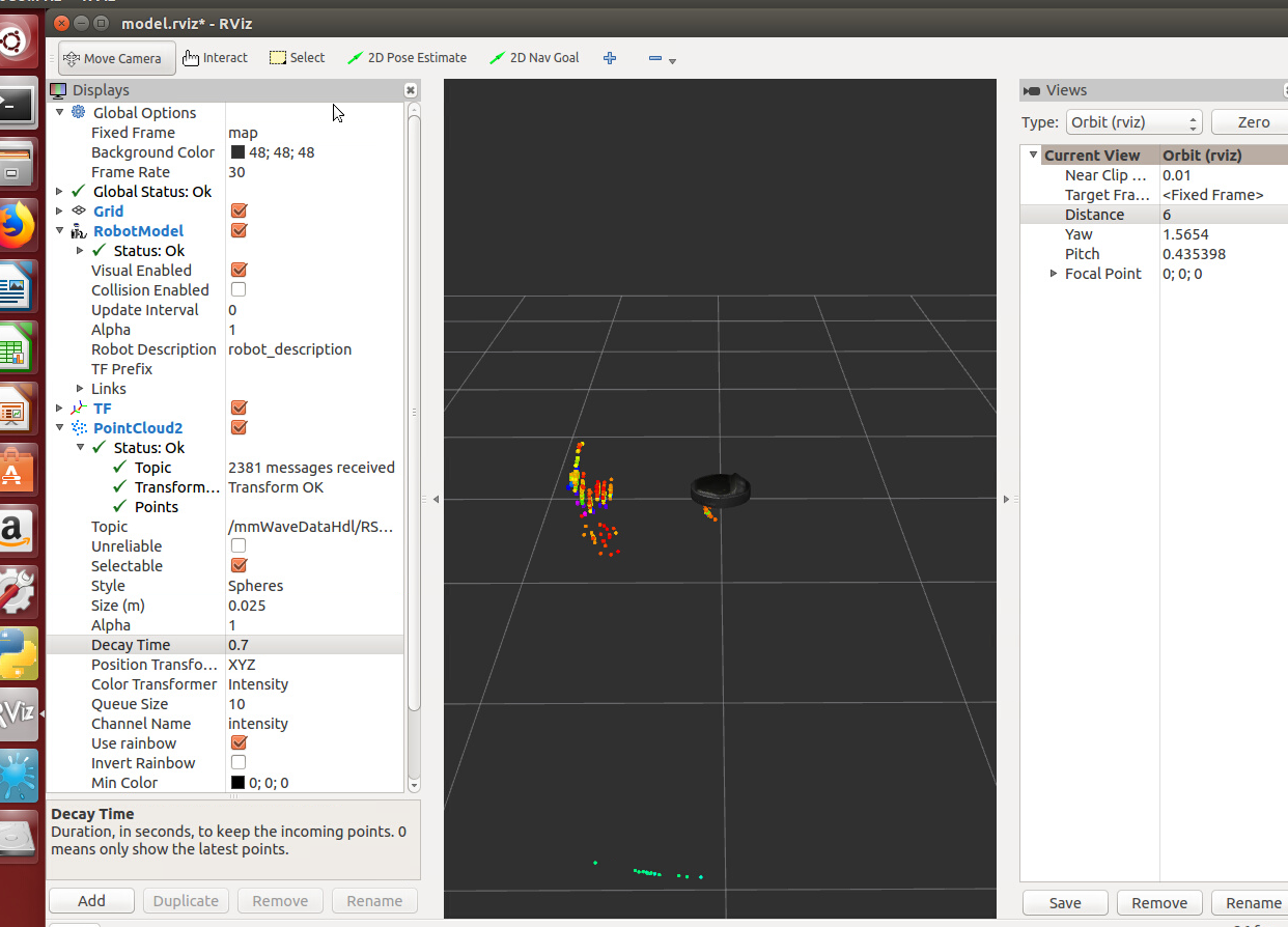
In RViz add point cloud from mmWave radar:
- Click Add->PointCloud2
- Select /mmWaveDataHdl/RScan from the Topic field dropdown for the PointCloud2 on the left hand panel
- Increase Size to 0.03, increase Decay Time to 0.25, and Select Style as “Spheres”.
- In rviz, select map for Fixed Frame in Global Options.
- If Kobuki is also started, set Reference Frame (left panel) to “map”.
You should see a point cloud image:
More information can be found in ROS driver document in chapters: “Visualizating the data”, “Reconfiguring the chirp profile”, and “How it works”
Starting GStreamer pipeline for streaming front view camer
It is possible to start GStreamer pipeline on Sitara and receive front-camera view on Ubuntu Linux box or Windows PC using VLC.
gst-launch-1.0 -e v4l2src device=/dev/video1  io-mode=5 ! 'video/x-raw, \
format=(string)NV12, width=(int)640, height=(int)480, framerate=(fraction)30/1' ! ducatih264enc bitrate=1000 ! queue ! h264parse config-interval=1 ! mpegtsmux  ! udpsink host=192.168.0.100 sync=false port=5000
E.g. on Windows PC (192.168.0.100), you can watch the stream using: “Program Files (x86)VideoLANVLCvlc.exe” udp://@192.168.0.100:5000
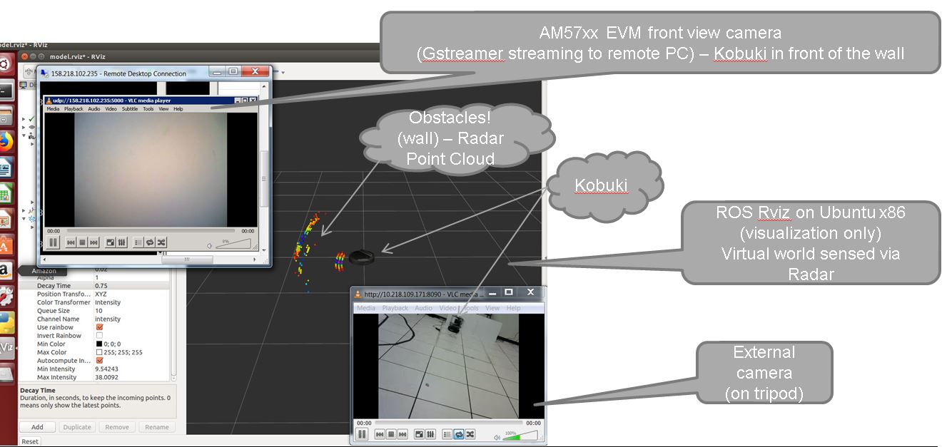
Fig. 5.7 Multiple windows on Ubuntu Linux box showing ROS RViz, front camera view and external camera view
5.3.11.6. Sense and Avoid Demo with mmWave and Sitara
Processor SDK Linux provides a complete sense and avoid navigation demo which runs on AM572x EVM with mmWave sensors. Details of this demo can be found from Autonomous robotics reference design with Sitara processors and mmWave sensors using ROS.
5.3.12. TIDL Classification Demo
Refer to various TIDL demos documented at Examples and Demos
5.3.13. Arm NN Classification Demo
Refer to Arm NN MobileNet Demo
5.3.14. Predictive Maintenance Demo
5.3.14.1. Introduction
Predictive Maintenance (PdM) promises to achieve levels of efficiency and safety on the factory floor never seen before in the current established best practices for systems and processes. Machine downtime is one of the biggest challenges on the production line. The current method of MRO (maintain, repair, operate) is far from what the optimum level of production can be. With predictive maintenance, once data is coming from equipment in real-time (or near real-time depending on application needs), advanced analytics are used to identify asset reliability risks that could impact business operations. By applying machine learning and analytics to operational data generated by critical assets to gain a better understanding of asset performance, companies can act on these insights as part of a continuous improvement process.
Predictive maintenance employs advanced analytics on the machine data collected from end sensor nodes to draw meaningful insights that more accurately predict machine failures. It is comprised of three steps: sense, compute and act. Data is collected from sensors that are already available in machines, by adding NEW sensors, or by using control inputs. Depending upon the machine types and the required failure analysis, different sensor signals – such as temperature, sound, magnetic field, current, voltage, ultrasonic, vibration – are analyzed to predict the failure. The predicted information from sensor data analysis is used to generate an event, work order and notification. The sensor data is also used to visualize the machine’s overall operating condition. An action is taken when the event reports an anomaly, a machine that is nearing the end of its useful life, or when wear and tear is detected in machine parts.
The following are the advantages of predictive maintenance using analytics:
- Detects incipient failures and breakdowns in early stages and facilitates early repair
- Establishes shelf life of asset and assesses product warranty
- Maintains inventory and tabs on spare parts
- Explores hypothetical scenarios
- Early notification and alerts to field operators and improves safety standards
- Prevents unnecessary downtime in production processes
- Maximizes lifecycle of equipment
- Enables product innovation . new features, services and pricing models
Some of the examples of predictive maintenance from real-life scenario includes:
- Find defective bearings long before defects are visually seen
- Find misalignment between two rotating pieces of equipment
- Recognize when fans become unbalanced
- Identify when bearings need lubrication
- Tell when an electrical connection needs to be tightened
- Alert when oil is contaminated or in need of replacement
An overview video for predictive maintenance can be found from predictive maintenance overview training.
Processor SDK Linux now provides a predictive maintenance demo which leverages Recurrent Neural Network (RNN) for anomaly detection over motor drive control. The sections below describes the demo in details, including the system model for anomaly detection with RNN, the workflow of developing the PdM demo with step by step instructions, the benchmarking results, and the PdM demo deliverables from Processor SDK Linux.
5.3.14.2. Anomaly detection system model with RNN
In addition to Convolutional Neural Network (CNN), recently RNN emerged as high-quality universal approximation method for time series. It is becoming more effective with many desktop tools supported by GPU acceleration.
For anomaly detection, a system model is established to predict the output from the input for the normal scenario. If prediction of the output values is good, the system model acts as a high-accuracy approximation of the physical system. With this system model, if there are significant and continuous prediction errors, it indicates anomalies are happening.

Fig. 5.8 System model for anomaly detection with RNN
5.3.14.3. Workflow for developing the PdM demo
The figure below illustrates the workflow for developing the PdM demo. It begins with acquiring data that describes the physical system in a range of healthy and faulty conditions. The data can be from sensors, or generated from a physical model. Then, the acquired data will go through some pre-processing, such as down-sampling to reduce the data dimension. After that, it comes to the stage of developing the model. For PdM, the model can be either a detection model for condition monitoring (e.g., anomaly detection) or a prediction model for prognostics (e.g., estimating the remaining useful life). The model development requires identifying appropriate condition indicators and then training a model to interpret these condition indicators. This is likely an iterative process, as you try different models and indicators and tune the model parameters such as the number of RNN layers and nodes. The last step is to deploy the model and integrate the solution into a system for machine monitoring and maintenance at the edge devices.

Fig. 5.9 Workflow for developing the PdM demo
In the following subsections, details are provided for the individual steps of this workflow using the anomaly detection for motor drive as the example.
5.3.14.3.1. Sensor data acquisition
In our PdM anomaly detection demo, the sensor data are originating from motor drive TI design. In this TI design, AM437x IDK (running Processor SDK RTOS, PRU-ICSS EtherCAT Slave, and PRU-ICSS Industrial Drives) is conducting motor control. It also receives the feedback about the phase current measurement and the position measurement. On the other hand, AM437x IDK acts as Ethercat slave and communicates with TwinCAT master on a host machine for setting the target velocity, target position, and etc.
To acquire the sensor data in real-time, high-speed (921600 baud rate) UART is implemented to send out the two phase currents (2 bytes each), and the motor position (4 bytes) with sampling rate of 10KHz. To get continuous sensor data, PyAutoGUI is employed to achieve automated control of TwinCAT, so that the motor can repeatedly move from position 1 to position 2, and then from position 2 back to position 1.

Fig. 5.10 Sensor data acquisition from motor drive
5.3.14.3.2. Sensor data pre-processing
For the sensor data with a frequency of 10KHz, simple pre-processing of low-pass filtering and down-sampling to 50Hz is done to reduce the high frequency noise. After that, normalization is done for the down-sampled sensor data.
Depending on the application, some Other preprocessing techniques can be applied, such as FFT, high order statistics, and wavelets.
5.3.14.3.3. Offline training to establish the model
To establish the RNN model, offline desktop training in MATLAB is done with the two down-sampled phase currents. The RNN topology contains a single Long Short-Term Memory (LSTM) layer, and a Fully Connected (FC) layer. There are 31 hidden nodes for the LSTM layer, and 31 inputs and 2 outputs for the FC layer. This is a simple RNN model, which is specified to avoid overfitting and control the computation load. The trained model is in Open Neural Network Exchange (ONNX) format. The last layer, regression layer, is the output layer used for prediction.

Fig. 5.11 Offline training RNN model with LSTM and FC layers
The RNN model is trained with the normal scenario data: motor moves with velocity of 100 degree per second from 45 degree to 270 degree and back to 45, and so on so forth. With a single training sequence about 50s long, the training with Matlab on a desktop PC is completed in less than three minutes.
Some other open source tools, such as Keras/Tensor Flow, Pytorch, can also be used for the training.
5.3.14.3.4. Deploy and integration
After getting the model, the last step is to deploy the model and integrate it for anomaly detection at the edge.
Build RNN inference library
To establish the RNN inference library implementing the LSTM and FC layers, our initial solution is using python scripts to convert the ONNX model into CPP header file, which contains the initialized data structures with all the weights information. The python scripts supports N stacked LSTM layers, plus one FC layer. The generated CPP header is then compiled with the LSTM library to create the ARMv7 object file with the initialization and processing APIs.

Fig. 5.12 Build RNN inference library
Real time anomaly detection at the edge
With the RNN inference library, we build the Linux user space application running on Arm to perform anomaly detection. The figure below shows the call flow of the anomaly detection. The two phase currents are received in real-time from the motor control application running on AM4 IDK. Then, low pass filtering and down-sampling are applied to the phase currents, followed by normalization. After that, RNN prediction is done upon the pre-processed phase currents, using the RNN inference library built above. The predicted phase currents are then de-normalized, and compared with the actual phase currents to calculate the prediction error. The prediction errors at the beginning for the normal scenario are used for calibration: the maximal prediction error in this stage is scaled with a ratio larger than 1 to be the anomaly detection threshold. After that, the prediction error will be used to report anomalies: if the prediction is larger than the threshold found in the calibration stage, then anomaly is reported.

Fig. 5.13 Real time anomaly detection
5.3.14.4. Deliverables from Processor SDK Linux
Processor SDK Linux provides an out of box PdM demo from Matrix GUI. It also supports re-building the demo from the top-level Makefile. Python-based conversion tool is also provided to convert an ONNX model into CPP header file.
5.3.14.4.1. Out of box demo with with pre-recorded sensor data
The PdM demo for anomaly detection is provided from Matrix GUI under Analytics submenu - PdM Anomaly Detection with RNN.

Fig. 5.14 PdM anomaly detection demo in Matrix GUI
For this out of box demo, pre-recorded sensor data (/usr/share/ti/examples/pdm/normal100-anomaly150-normal100.log) is used as the testing sequence, as shown in the demo scripts (/usr/bin/runPdmAnomalyDetection.sh). This testing sequence starts with the normal scenario data, i.e., motor moves with velocity of 100 degree per second from 45 degree to 270 degree and back to 45, and so on so forth. To create anomalies, the motor moves with a higher velocity of 150 degree per second after some time. The figure below shows the Qt GUI display of the demo. The left-side panel shows the real-time sensor input: the two phase currents in blue and green, and the motor position in orange. The right-side panel shows the detection results: the blue line is the anomaly detection threshold found from the calibration, the orange line draws the prediction error, while the red line draws the time period of the detected anomaly.

Fig. 5.15 Anomaly detection demo display
Filesystem of Processor SDK Linux also packages two more pre-recorded testing sequences (under /usr/share/ti/examples/pdm/), for some other anomalies.
- normal270-anomaly170-normal270.log: motor moving from 45 degree to a different (170 instead of 270) degree.
- normal45-270-v100-with-friction2-iter10-15.log: hand-pressing the coupler between the motor and the encoder to add more friction.
5.3.14.4.2. Support rebuilding the demo from top-level Makefile
The source of the PdM demo for real-time inference is available at pdm-anomaly-detection git rep. The source is also bundled with Processor SDK Linux installer, under the example-applications directory:
[plsdk_install_dir]/example-applications/pdm-anomaly-detection-1.0
Rebuilding of the demo can be done via the top-level Makefile of Processor SDK Linux:
cd [plsdk_install_dir]
make pdm-anomaly-detection
After the compilation is completed, the demo binary can be found at [plsdk_install_dir]/example-applications/pdm-anomaly-detection-1.0/RnnPdmAnomalyDetection.
5.3.14.4.3. ONNX model conversion tool
Python scripts are provided in the PdM demo source under the model folder to convert ONNX model to CPP header file with initialized data structures. It supports N stacked LSTM layers plus on fully connected layer as the last layer.
Before running the scripts, install the python packages below if this has not been done earlier.
sudo apt install python-pip
pip install numpy pandas scipy onnx
Then, run the command below to do the conversion:
cd pdm-anomaly-detection/model or pdm-anomaly-detection-1.0/model
python ./make_header.py -m ./[onnx-model-file]
The output CPP header file is called LSTM_model.h which is placed under the same model folder.
5.3.14.5. Benchmarking for anomaly detection with RNN
To conduct benchmarking for the RNN based anomaly detection, two threads are used with Qt/QML display not in the picture.
- thread 1: main processing thread with RNN prediction and anomaly detection
- thread 2: parsing thread to read senor data
Linux clock_gettime() function is used for reading the time:
clock_gettime(CLOCK_REALTIME, &ts0);

/* Run LSTM network for prediction */
runLstm(lstm_in1, lstm_in2, &lstm_out1, &lstm_out2);

clock_gettime(CLOCK_REALTIME, &ts1);
ns_lstm = (ts1.tv_sec-ts0.tv_sec) * 1000000000 + ts1.tv_nsec-ts0.tv_nsec;
Two benchmarking points are used:
- Pre-processing: low-pass filtering and down-sampling to reduce 200 samples to 1 sample
- RNN prediction (LSTM + FC) on 1 sample
Average compute time per sample:
- RNN prediction: 0.083ms
- Pre-processing: 0.014ms
- Total (RNN prediction and pre-processing): 0.097ms
With a sampling rate 50Hz, RNN based anomaly detection consumes around 0.5% of CPU running at 1GHz, showing a low computation load.
5.3.15. PRU-ADC Demo
5.3.15.1. Introduction
This demo shows flexible interface for Simultaneous, Coherent DAQ Using Multiple ADCs via PRU-ICSS. More details can be found at https://www.ti.com/tool/TIDA-01555
5.3.15.2. Hardware Needed
Please refer to the TI Design to set up the hardware needed to run this demo.
- Beaglebone Black
- TIDA-01555 adapter card
- TIDA-01555 ADC board
- Desktop power supply to provide 5.5 volts to the ADC board
- Desktop signal generator to produce a 45-55Hz sine wave as an input
5.3.15.3. Steps to Run the Demo
Below are the steps to run the demo with Processor SDK Linux RT build for AM335x.
First, use /boot/am335x-boneblack-pru-adc.dtb as the default dtb:
cd /boot
cp am335x-boneblack.dtb am335x-boneblack.dtb.orig
cp am335x-boneblack-pru-adc.dtb am335x-boneblack.dtb
Then, link am335x-pru*_fw to the PRU-ADC firmware binaries:
cd /lib/firmware
ln -sf /lib/firmware/pru/PRU_ADS8688_Controller.out am335x-pru0-fw
ln -sf /lib/firmware/pru/PRU_ADS8688_Interface.out am335x-pru1-fw
After that, reboot the EVM, and then execute the ARM binary:
run-pru-adc.sh
5.3.16. Video Graphics Test
5.3.16.1. Introduction
The video graphics test application demonstrates various video processing, graphics and display capabilities using VIP, GC320, SGX and DSS IPs. Many embedded applications need multiple displays with multiple videos and graphics planes rendered on different screens. Such applications can be developed with or without using a windowing system like Wayland. Using a windowing system demands more system resources like CPU, GPU and DDR bandwidth and increases system complexity. When the system resources are in a crunch and there is no real need to use a windowing system, many users prefer to use no windowing system (alternately called as NULL window or full-screen mode). The video graphics test application demonstrates such application development in full-screen mode using QT.
QT framework is a popular tool to draw the software or hardware accelerated graphics contents. It can manage the display backend of embedded Linux system to render the contents in full-screen mode. It provides creation of a full-screen window by platform-specific means, known as QT Platform Abstraction (QPA). EGLFS is a platform plugin for running Qt5 applications on top of EGL and OpenGL ES 2.0 without an actual windowing system. When having multiple displays connected, QT provides another plugin named eglfs_kms to render the content on multiple displays. In eglfs_kms QPA, DRM Linux Kernel Mode Setting (KMS) API is used to set DSS mode. By default, eglfs_kms provided by QT doesn’t take advantage of the advance capabilities of DSS IP such as scaling, overlaying and alpha-blending of the videos/graphics planes.
To enable optimal usage of all the IPs on the AM57x8 devices and to deliver the best performance while running the QT application, we have enhanced the eglfs_kms QPA to leverage the DSS IP advance capabilities. The QPA exposes many callback functions through QPlatformNativeInterface to allow the users to set DSS IP advance properties. This enhanced QPA is packaged in PSDK Linux filesystem.
5.3.16.2. GC320 Usage for Rotation, Composition, Overlaying and Alpha-Blending
GC320 is the 2D graphics accelerator from the Vivante Corporation and the IP is capable of performing tasks such as scaling, bit-blitting, rotation, composition, alpha-blending and many other 2D processing. Please refer to the Technical Reference Manual for the SOCs to learn about the capabilities of the GC320 accelerator.
DSS IP can accept up to 4 videos and graphics planes as input and send them individually or as overlaid/composed frames to different display monitors. If the application needs to display more planes than what DSS can accept, then it is recommended to use GC320 for composition/overlaying of some of those planes before sending to DSS. In the video graphics test application, we demonstrate GC320 usage for video scaling, rotation and overlaying/composition feature.
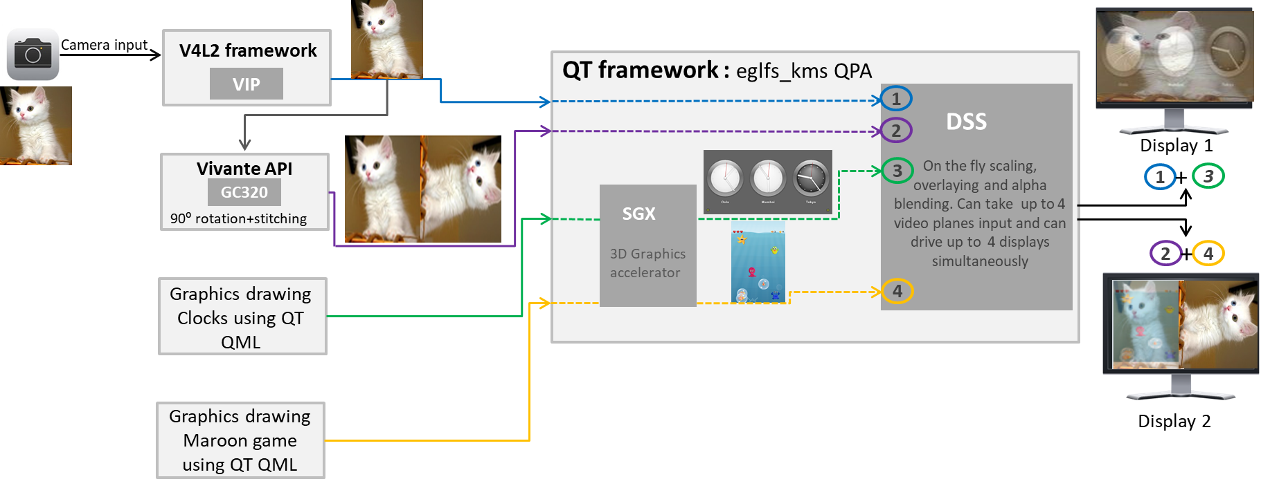
5.3.16.3. Application Description
In the video graphics test application, we have demonstrated embedded application displaying two different videos and graphics contents rendered on two different display monitors in full-screen mode. One of the video sources comes from camera input hooked to parallel capture port VIP. Captured video is submitted to QT eglfs_kms QPA to be rendered on Display1 device. Next, the application takes the relevant information from the camera input and passes two copies of the same image to the GC320. The GC320 takes one copy and does not modify the image. For the second copy, the GC320 will rotate the image by 90 degrees. Then, the GC320 will stitch both images together and the output is submitted to QT plugin for rendering on Display2 device. QT framework is also used to draw analog clock and Maroon game using QT QML. The analog clock is set to be rendered on Display1 and Maroon game to be rendered on Display2. QT uses OpenGL APIs to render the graphics contents using 3D graphics accelerator SGX544. The users submit the properties of video planes like scaling, overlaying, alpha-blending, number of display monitors and etc using the APIs exposed through QPlatformNativeInterface. It sets the video planes to blend with graphics planes and the resulting output renders to the size of the display on both the monitors. QT uses DSS hardware accelerator to accelerate the overlaying, alpha blending and scaling processing.
Video Graphics Test Block Diagram
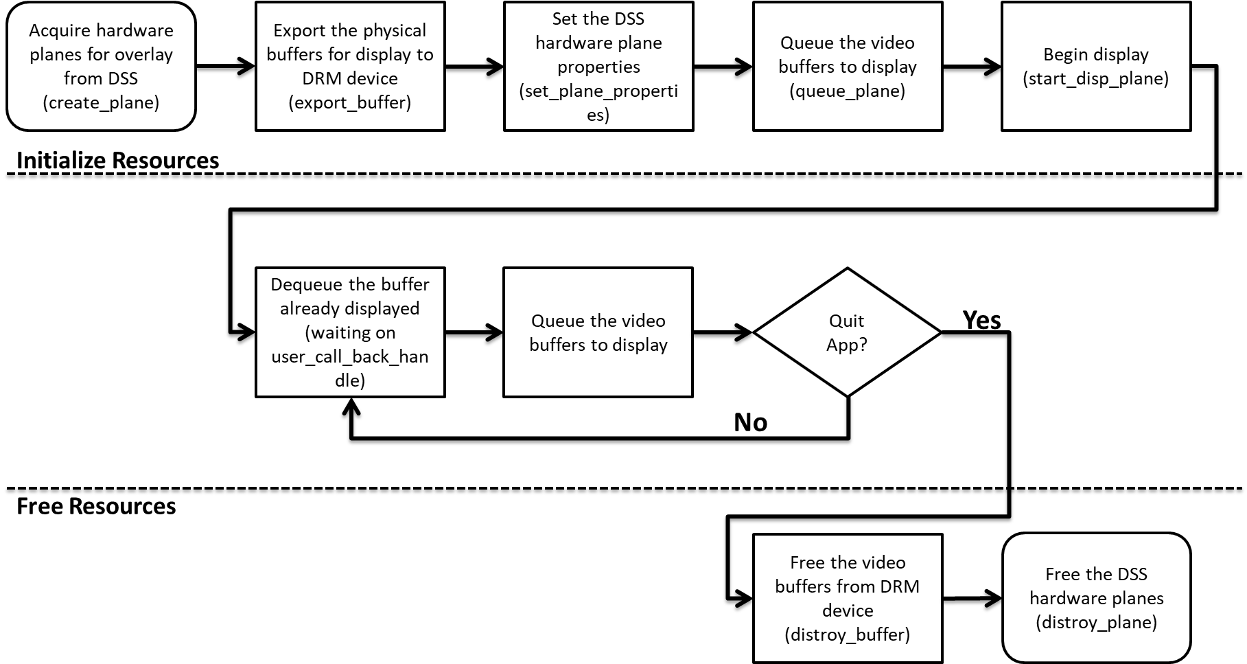
5.3.16.4. eglfs-kms QPA User Exposed APIs
As part of eglfs_kms QPA enhancement, following APIs are exposed via QPlatformNativeInterface to allocate DSS hardware planes, to set the plane properties supported by DSS and to submit the buffer for display.
1. create_plane: Secure DSS hardware planes for overlay from QT QPA
2. distroy_plane: Free the reserved DSS hardware planes
3. export_buffer: Export user allocated buffer to the QT QPA
4. distroy_buffer: Free the buffers
5. set_plane_properties: Set the DSS plane properties for scaling of video planes and blending it with graphics planes. Properties can be set for both DRM plane type Primary and Overlay planes.
6. get_plane_property: Read default/pre-set property value of a plane
7. queue_plane: Queue the video buffer to a QPA plane to be overlayed/displayed
8. start_disp_plane: Begin displaying of the queued buffers
9. user_call_back_handle: Pass callback function pointer to the QT eglfs_kms QPA. The QPA will call this function to notify user the display completion of the overlay buffer
The APIs required to achieve scaling, overlaying and alpha-blending using the DSS IP owned by eglfs_kms QPA are demonstrated inside disp_obj.cpp and video_graphics_test.cpp file. An example of the software flow is shown below:
5.3.16.5. Running the Test
In order for the users to run the video graphics test, please type the following commands on the EVM:
target # insmod /lib/modules/<kernel_version>/extra/galcore.ko baseAddress=0x80000000 physSize=0x80000000
target # /etc/init.d/weston stop
target # export QT_QPA_EGLFS_INTEGRATION=eglfs_km
target # video-graphics-test -platform eglfs
5.3.17. Watchdog Demo on AM654x PG 1.0
5.3.17.1. Introduction
The traditional watchdog with SoC/core reset capability on Linux is not supported on AM654x PG1.0 due to hardware limitation. In stead, the following workaround is implemented to demostrate the tranditional watchdog functionality as described and shown below.
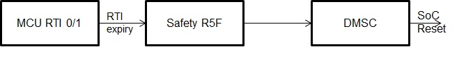
- Standard Linux watchdog with MCU RTI0/1 in kernel
- Linux watchdog daemon configures watchdog timeout, strats and feeds the watchdog periodically
- The RTI expiry interrupt is fed into the Safety R5F where the demo firmware instructs DMSC to trigger SoC reset when RTI expiration interrupt is detected.
5.3.17.2. Running the Demo
In order for the users to run the watchdog demo, follow the following procedure on the AM654x PG1.0 platform:
- Replace the IPC firmware with the wdt test firmware
target # ln -sf /lib/firmware/rti_dwwdtest/am65xx_evm/csl_rti_dwwd_test_app_mcu1_0_release.xer5f /lib/firmware/am65x-mcu-r5f0_0-fw
- Reboot and run the Watchdog demo by starting watchdog
target # watchdog
- Do normal operations
- Stop watchdog daemon and observe the system reset occurs within 2-3 minmutes
target # pkill watchdog
- Restore the IPC firmware after SoC reboot
target # ln -sf /lib/firmware/ipc/ti_platforms_cortexR_AM65X_R5F0/messageq_single.xer5f /lib/firmware/am65x-mcu-r5f0_0-fw