|
Vision Apps User Guide
|


|
|
Vision Apps User Guide
|
|
The tasks involved in Autonomous/Automated Driving (AD) can be categorized in 4 modules of 1) perception, 2) localization 3) mapping and 4) planning and control. The localization module determines position of the vehicle i.e. 3D location and orientation and plays a critical role in safe and comfortable navigation. Localization is the process of estimating vehicle position in the paradigm of map-based navigation. When localization process uses only camera sensor it is referred to as Visual Localization. Visual localization is particularly valuable when other means of localization are unavailable e.g. GPS denied environments such as indoor locations. Also Visual Localization output can be fused with noisy Inertial Navigation System(INS) to obtain overall accurate vehicle positions. Along with self-driving cars other applications include robot navigation and augmented reality.
| Platform | Linux x86_64 | Linux+RTOS mode | QNX+RTOS mode | SoC |
|---|---|---|---|---|
| Support | YES | YES | YES | J721e / J721S2 / J784S4 |
The example Visual Localization (VL) scheme performs 6-Degrees of Freedom ego-localization using 3D sparse map of area of automated operation and a query image. Each point in the sparse map stores visual and location information of the scene key-point which can be used at localization time to match against the key-points in the query image. The Visual Localization process thus is built around camera pose estimation approach such as Perspective-n-Point (PnP) problem. PnP is the problem of estimating the pose of a calibrated camera given a set of n 3D points in the world and their corresponding 2D projections in the image. Considering the perspective transform as defined in equation below the problem then is to estimate the rotation and translation matrix [R|T] of the camera when provided with N numbers of world(Pw) - camera(Pc) point correspondences.
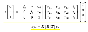
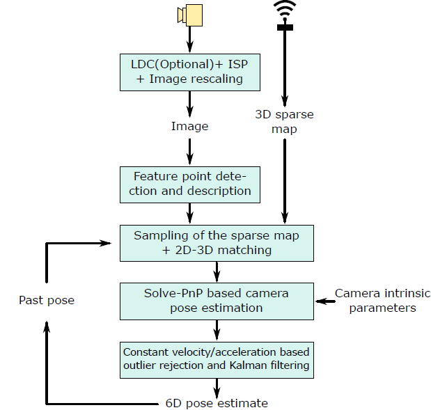
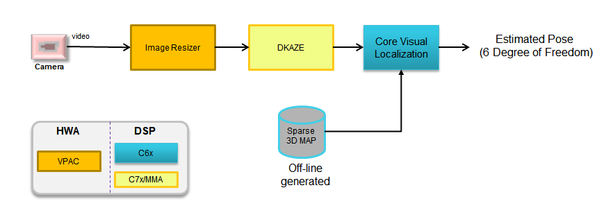
The [R|T] matrix encodes the camera pose in 6 degrees-of-freedom (DoF) which are made up of the rotation (roll, pitch, and yaw) and 3D translation of the camera with respect to the world. The VL process thus involves detection and description of key-points points in the query image captured by the onboard camera of the vehicle, matching of the 2D image points with that of 3D landmark points from map to establish 2D-3D point correspondences, followed by camera-pose estimation using any of the SolvePnP solutions. This simplified process is depicted in the following Fig. Offline calibration of the camera sensors and vehicles frame of reference provides the extrinsic parameters that can be used to estimate the vehicle pose from the estimated camera pose.
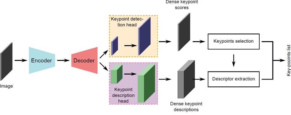
Key-point Descriptor plays critical role in ensuring high accuracy during Visual localization process. However descriptor computation can put quite a load on compute resources like CPU/DSPs. To address this issue we adopt Deep Learning based approach. We train deep neural net (DNN) to learn hand computed feature descriptor like KAZE in a supervised manner. We refer such descriptor as DKAZE. As DKAZE uses very similar network architecture as typical semantics segmentation networks, in actual deployment DKAZE can be considered as an additional decoder in multitask network (single encoder + multiple decoders topology).
Along with the out-of-box example, dataset generated using Carla Simulator 0.9.9.4 (https://carla.org/) is provided. Dataset contains the following,
The snapshot of one of the captured images is shown below.
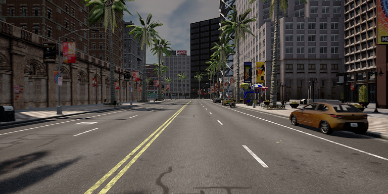
We also make Python script to capture dataset using Carla available on request.
The following is the X-Z plot of the localization position estimates of vehicles with ground truth vehicle positions. It is evident that visual localization output is very close to ground truth locations. Also it is able to handle sharp turn without any issue.
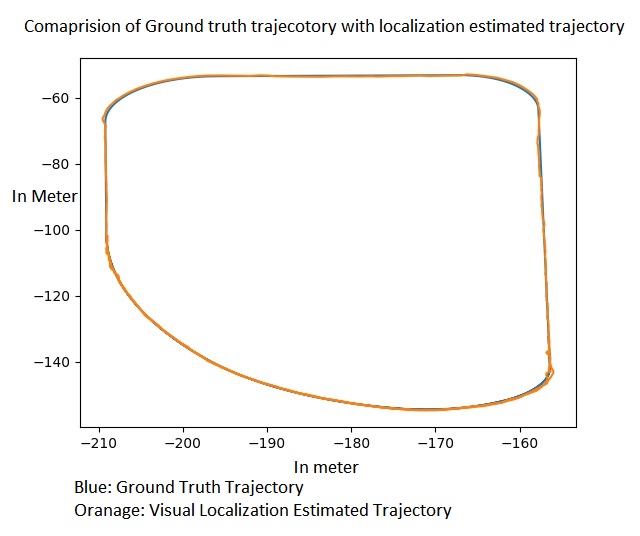
Here is the objective comparison with GT positions,
| use-case | Average error |
|---|---|
| 10 fps | 16.3 cm |
| 30 fps | 10.6 cm |
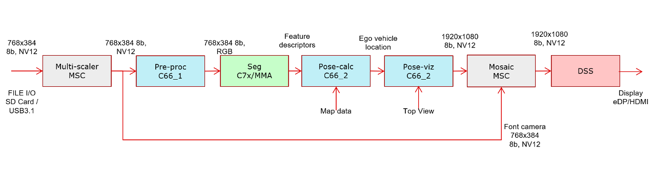
The following conceptual block diagram indicates where various components of visualization location pipeline get mapped to various HW resources available on SOC.
In this demo, we read file based NV12 inputs of resolution 768x384 from SD card and pass it to a resize MSC. As the input resolution is matching with resolution required by DKAZE network, the input and output resolution of resizer stage is the same. This is then passed to C66x_1 for pre-processing where NV12 image is converted to RGB/BGR planar image along with necessary padding as required by TIDL. The DKAZE features are then obtained from TIDL running on C7x and is passed to C66x_2 for pose calculation. The result is then sent to another OpenVx node running on the same C66x_2 core for visualization where the position of the car is indicated by a blue pixel. The intensity of the pixel changes as the ego vehicle moves. This information is overlayed on the top view of the map and passed to SW mosaic node for overlay with front camera image on a 1920x1080 NV12 plane. This plane is submitted to DSS for display.
During localization deployment per Kilometer MAP size is one of the critical factors to ensure real time operations. We adopt sparse 3D format for the Map storage, which does not need camera images, resulting in more compact MAP size. With out-of-box visual localization example, the off-line created sparse 3D map is provided. One can create her own off-line map in the following format,
An example map file,
As an out-of-box example end-to-end optimized visual localization pipeline SW is provided. However one can build her own pipeline by either replacing few compute blocks of her own choice or create visual localization pipeline from scratch but accelerate compute heavy blocks by utilizing available optimized blocks. The following are the optimized compute blocks are available as part of TIADALG component package.
1. Two Way Descriptor Matching -
Name of the API: tiadalg_select_top_feature()
This API can be used to carry out two way matching between 2 sets of descriptors. Typically descriptors sample form the sparse 3D map and descriptors computed using current frame need to be matched to find N best matching pairs. This API does two directional matching to avoid wrong matches resulting from feature less regions like flat surfaces. It supports unsigned 16 and unsigned 8 bit descriptors datatype. Length of descriptor is configurable. The current example exercises 8 bit unsigned type descriptor with 64 elements per descriptor.
2. Sparse Up-sampling -
Name of the API: tiadalg_sparse_upsampling()
DKAZE module generates the descriptors at 1/4th image resolution for optimal memory usage. However Visual localization pipeline needs it at full resolution. To do up-sampling process in most optimal manner this API does up-sampling only on the sparse points selected by key point detector using nearest neighbor resizing. It also applies 7x7 filtering on the resized data.
3. Recursive NMS -
Name of the API: tiadalg_image_recursive_nms()
DKAZE module produces key point score plane buffer at original image resolution. It does scores plane buffer thresholding, and then 3x3 NMS is performed on thresholded score buffer. This is helpful getting relevant interest points in the scenario where scores are saturated in clusters. These compute blocks executes on C66x DSP as part of visual localization OpenVX node.
4. Perspective N Point Pose estimation, a.k.a. SolvePnP -
Name of the API: tiadalg_solve_pnp()
After establishing 2D-3D correspondences using, two way descriptor matching API shown above, one can use perspective N point API to find 6 DOF camera pose.
More details about these API interfaces and compute performance details are provided in user guide and data sheet of TIADALG component.
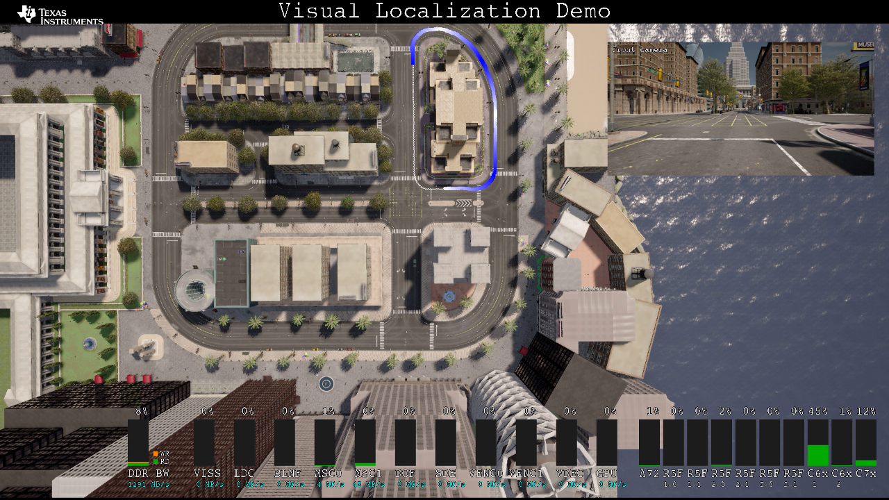
The following picture shows trajectory of estimated positions generated using visual localization (thick blue line) on the top-view image. The thin white line indicates ground truth trajectory.
 1.8.14