|
Vision Apps User Guide
|


|
|
Vision Apps User Guide
|
|
The tasks involved in Autonomous/Automated Driving (AD) can be categorized in 4 modules of 1) perception, 2) localization 3) mapping and 4) planning and control. The perception module may include task to find obstacles directly in the path of driving. This can be achieved using sparse 3d points generated for surrounding environment using computer vision based technique Structure From Motion (SFM).
In Computer Vision, the position of an object with respect to a vehicle is ascertained using images from two cameras, mounted on known disparate locations, looking at the object in question. In particular, key points from the object in both images are extracted and matched, and then using a process known as Triangulation, the locations of the points that make up the object are deciphered. The process of distinguishing the position of a point in space using two cameras is known in the Computer Vision community as Stereo Vision, or Stereo Depth Estimation, and the set of points generated from all the correspondences in the two images is referred to as a point-cloud.
Even as Stereo Vision is widely used by the automotive and industrial communities, it comes at a high system cost in terms of both dollars and image processing requirements, because it requires two high-precision cameras, capturing images at a relatively high frequency.
In contrast, Structure From Motion, or SFM, is an algorithm that can generate a point-cloud from a monocular camera in motion. As the name implies, in SFM, we have single camera which due to the motion is in two distinct locations at two consecutive time instances, which effectively similar to placing two cameras in distinct locations for static structures and obstacles. Thus, one can effectively use the same theory as in Stereo Vision to generate a point-cloud, from just one camera.
SFM algorithms come in two primary flavors, traditional Computer Vision based and Deep Learning based. Even though both flavors can be executed on TDA4VM, in this application we focus on the former, an algorithm based on traditional Computer Vision techniques and how the algorithm can be efficiently executed using the Hardware Accelerators on the J7/TDA4VM device.
Establishing point correspondences between images is central for realizing SFM for real time applications. To accelerate this process Texas Instruments Jacinto7 family of SoCs like J721e/TDA4VM introduces on chip hardware accelerator (HWA) called Depth And Motion Accelerator (DMPAC). The DMPAC contains Dense Optical Flow (DOF) HWA which can be used to establish point correspondences without burdening DSP or CPUs (MPU). TI-DOF can perform more than 120 Mega pixel per second dense optical flow.
DOF needs generation of multi scale inputs for generating high quality optical flow even in case of large motion due to fast moving vehicle or to capture close by object. To facilitate this Jacinto7 family of SoCs like J721e/TDA4VM contains Hardware accelerator called Multi Scaler as part of VPAC block.
| Platform | Linux x86_64 | Linux+RTOS mode | QNX+RTOS mode | SoC |
|---|---|---|---|---|
| Support | YES | YES | YES | J721e / J721S2 / J784S4 / J742S2 |
The following conceptual block diagram indicates where various components of visualization location pipeline get mapped to various HW resources available on SOC.
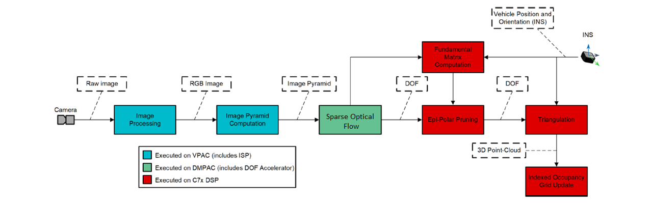
In this demo, we read file based Luma inputs of resolution 1024x512 from SD card and pass it VPACK h/w to generate 4 level of image pyramids. At each pyramid level image resolution drops by 2x in both x & y direction. These pyramid images are fed to DOF h/w accelerators to compute optical flow information for all the pixels. Key points are inserted at regular grid of 8x8, and these key points are tracked using the optical flow information up to maximum last 6 frames. Followed by triangulation and various error checks 3d points are generated for each track. Later occupancy grid is created using these 3d points.
This 3d point information is overlaid with input image is done on C7x. Occupancy grid visualization is created inside core SFM algorithm executing on C7x node. The visualization buffer of 3d point cloud and occupancy grid is passed to SW mosaic node for creating single plane of 1920x1080 resolution. This plane is submitted to DSS for display.
Occupancy Grid Maps are a widely used method to represent the environment surrounding a vehicle or robot, because they can be consumed by a variety of ADAS applications ranging from parking, to obstacle identification, to curb detection, and be stored efficiently. An Occupancy Grid map, or OG map, is a representation of a vehicle’s surroundings in the form of a 2-Dimensional or 3-Dimensional grid. Each grid cell in the map has a corresponding state, for example Occupied, Free or Unknown, computed using information received from sensors such as Radars, Cameras, or LiDARs. A simple illustrative example of an OG map is shown below in Figure.
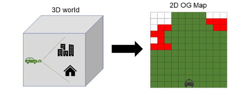
OG maps can either be centered on the vehicle or robot, or centered on an arbitrary frame of reference. The former is known as an ego-centric OG map and the latter as a world-centric OG map. OG maps are further categorized as accumulated or instantaneous, based on whether or not information from previous frames is used.
As an out-of-box example end-to-end optimized structure from motion pipeline SW is provided. However one can build own pipeline by either replacing few compute blocks of her own choice or create structure from motion pipeline from scratch but accelerate compute heavy blocks by utilizing available optimized blocks. The following are the optimized compute blocks are available as part of TIADALG component package.
1. Track Formation from Optical Flow -
Name of the API: SFM_TI_updateTrack()
This API can be used to make tracks from the optical flow information. New keypoints are inserted as regular grid interval, and they are tracked upto maximum last 6 frames using the optical flow information generated for DOF hardware.
2. Finding a 2d point is inlier or outlier based on Epipolar geometry check -
Name of the API: VXLIB_FMAT_mapPoints_ci()
Validate the optical flow information based on Epipolar geometry check using Fundamental matrix.
3. Triangulation -
Name of the API: VXLIB_triangulatePoints_i32f_o32f_kernel()
Does the core 3d point generation from track information. Each track results in one 3d point.
4. 3D point reprojection on image plane error calculation -
Name of the API: SFM_TI_reprojErrorCalc_ci()
Re-projects the 3d point on image plane, and calculate the error between the re-projected point and original image points from which this 3d point got generated.
5. Calculating occupancy grid from 3d point cloud -
Name of the API: SFM_TI_genOccpGrid_ci()
This API generates the occupancy grid information from generated 3d points.
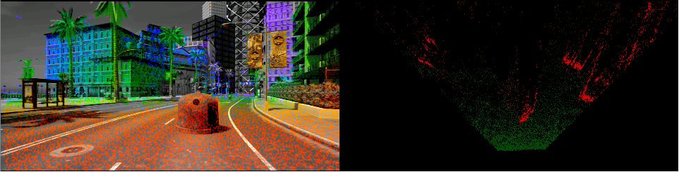
The following picture shows one frame output from out of box SfM application. Left picture shows reconstructed 3d points overlaid on image, and right picture shows occupancy grid in top view. Color notation in left image is in reverse VIBGYOR pattern, this means nearest 3d point is shown in red color whereas farthest 3d point is shown in violet color. In right image, red color indicates obstacle, whereas green indicates free space. This output is generated for 1024x512 image resolution, with 20k tracks.
 1.8.14